This document provides a brief introduction to BrainSpinner, instructions on how to use it and navigate through the menus, and a comprehensive demonstration of most of the features.
Introduction:
BrainSpinner is a display and interrogation program for anatomic and functional brain data. It can simltaneously display:
The brain surface can be made semi-transparent, and you can select a threshold to define the surface. You can add and remove any of the component items (box, marker, brain surface, slice views on back walls, cut views inside brain, functional volumes) without affecting other items. There are several options for each item like color, opacity, appearance, etc., and the various objects are displayed simultaneously.
You can obtain information about the underlying pixel values for any of the volumes by clicking on one of the orthogonal planes, or on the surface of one of the objects. If the ORIGIN values are set in the ANALYZE .hdr field, then the text-widgets on the left display the actual location and value(s) for each volume.
I use BrainSpinner to get a "big-picture" view of my data, to combine several modalities/scans, and to make groovy pictures for publications. You may find it helpful to print a hardcopy of this help-file, so you can go through some of the subsequent demos and examples.
File Format:
BrainSpinner requires its input data to be in the ANALYZE file format. This is the standard format used by SPM, AIR, and SPAMALIZE. The data that are read into the "Anatomy" volume defines the dimensions of the display space. Any subsequent volumes used (e.g. Mask, Functional, etc.) must have the same physical dimensions (number of pixels), otherwise BrainSpinner will refuse to read it! If only the pixel dimension (mm) is different it will not matter. The key information in the .hdr file are the dimensions (pixels), the pixel dimensions (mm), the calibration factor (funused), and the type (integer, floating etc.) which defines the number of bits/pixel.
BrainSpinner does pay attention to the pixel dimension, so if the .hdr file does not contain the correct pixel dimensions the aspect ratio will be wrong.
User Instructions:
Left mouse is for the pseudo-trackball. Click, drag, release in the brain window to spin the brain.
Right mouse is to select a point from the brain surface or the back image planes. Selecting a point changes the current pixel location and causes at least one of the planar views to be updated. You can actually click on any volume object to move the current location.
Data values: the actual values of the underlying data at the current location are displayed in the upper portion of the left panel.
Location: The location is displayed in the left panel in the center. The top location is pixels from the first corner (row, column, plane). The lower 2 locations assume that the ORIGINATOR field in the ANALYZE .hdr has been set to some value that makes sense, like at the anterior commisure. The location is given in terms of mm and pixels from the ORIGIN. You can type a value into any of these fields, if you have a particular location in mind. Click on the labels (Up/Down, etc.) in the small window for finer control over plane movement.
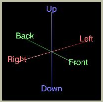
The 3D axis in the upper right corner indicates the orientation, and by clicking on the words ("Front", "Back", etc.) with the right mouse button you can move the current location (and hence the displayed slices) by an increment of one (1).
The middle section of the right panel contains all of the parameters for the various elements. Click on the dropdown menu labeled "Parameter For: .. Slices" to see the full range of options. Selecting an option causes the relevant parameters for that item to appear in the menu box.
The upper right hand panel lets you set lower-level thresholds for various volumes. This can be helpful, for example, if you want to exclude CSF from the edge of a T1-weighted MRI brain volume, to reveal the folded sulcal/gyral structures of the brain surface.
Resize the main window by clicking on the lower-left (or lower-right) corner of the main GUI, and dragging it up/down to the desired size. The main display window is limited to a square shape.
Demo/Tour:
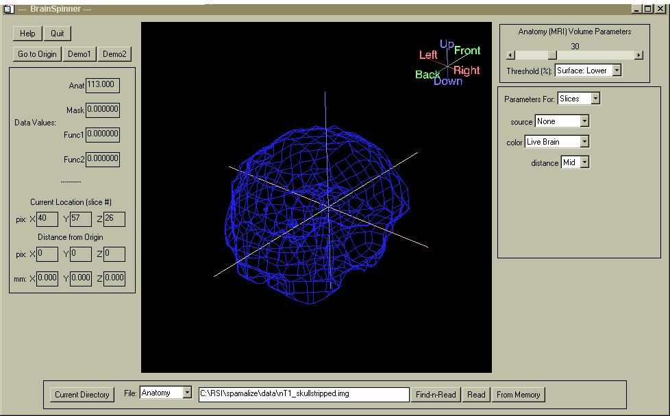
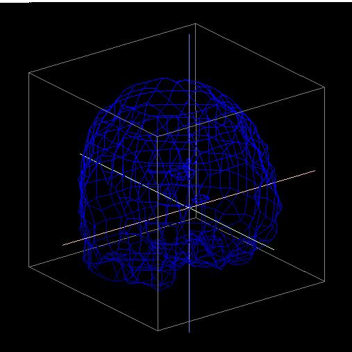
Type "spam" (assuming you installed SPAMALIZE according to the instructions) and go to "Toys -> BrainSpinner". A scalp-peeled MRI will automatically be loaded from the SPAMALIZE data directory. A blue mesh outline of a brain should be in the main window, as shown above. You can load in any other image volume you want into the "Anatomy" volume, by clicking on the "Find-n-Read" button in the File menu, as shown below. If the desired image file has different X,Y,Z dimensions than the currentl Anatomy volume, then all of other image volumes you may have loaded (Mask, Functional, etc.) will be discarded. You will be warned about this in a popup menu- if you are sure you want to load the new volume, click "Yes".

For this demo we will use the default volume, which is the canonical T1 MRI image from SPM96, normalized to the MNI bounding box with pixels size 2x2x2mm.
First of all, click on the "Demo" button in the upper left corner of the menu (not shown in picture above). This puts BrainSpinner through its paces, and will show you a lot of the various features in one fell swoop. When the demo is over, quit out of BrainSpinner and re-start it, to reset all of the parameters to their original values.
Use the right mouse button as a virtual trackball to move the brain to the following approximate location, with the front of the brain pointed toward the lower right face of the cube as shown below:
 |
|
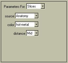
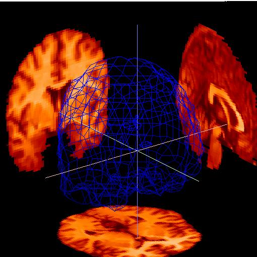
Go to the "Parameters for .. Slices" dropdown menu as shown below. Select "source .. Anatomy", which will display the MRI slices on the back walls. Change the color of the slices by selecting "color .. hot-metal". Go to "Parameters for: .. Box" and select "style: .. None" to remove the box. You should have an image like the following:
 |
 |
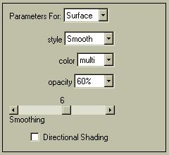
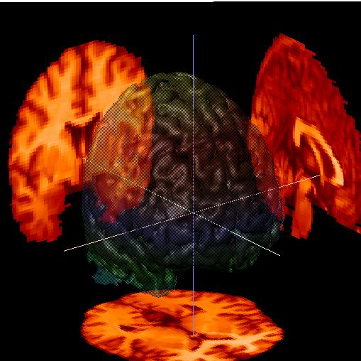
Let's try to show the beautiful wrinkles of the brain surface to a greater advantage. Go to "Parameters for: .. Surface" and select "style .. Smooth", "color .. multi" (from the color chooser menu, see below), and "opacity .. 60%" as shown in the menu below. You should get the following image:
 |
 |
You can choose from any of these surface types:
The "Smooth" surface takes a couple of seconds to create, which can seem like a long time in an interactive program. Most of the time is spent calculating the light-paths needed to give a realistic appearance. When you move a "Smooth" image with the trackball, the appearance will revert to the previous display type (usually Wire Mesh) which will give a real-time display during the motion, and will then create the new "Smooth" image when you release the mouse button.
The "opacity" parameter lets you create a semi-transparent brain surface, with obects inside of or behind the brain remaining visible. Select "60%" to emphasize the brain surface, or "30%" to emphasize the objects. Select "invisible" to hide the brain surface, or "opaque" to make it a solid surface.
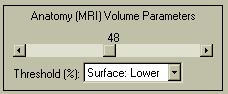 |
In order to show the brain surface as in the image above, you will have to modify the threshold used to define the surface. Change the "Surface: Lower" threshold (the default) from 30 to 48, as indicated at the left. The value indicates the percentage of the range of MRI values (max-min) that will be excluded from the brain surface. Higher values will accentuate the surface. |
Color Chooser:
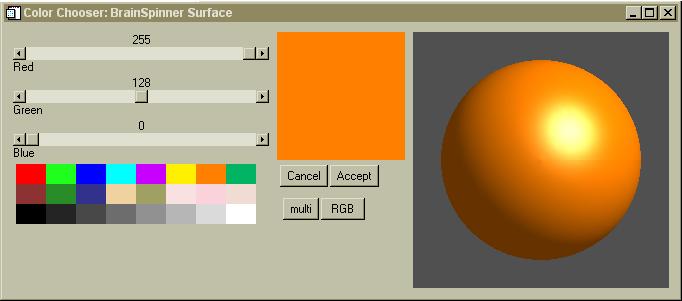
Many of the objects have their color set through the color chooser menu shown above. If the object can be rendered in 3D, it will show the 3D sphere so you can see how a color will look. If it is not a 3-dimensional rendered object (like a simple line) then the sphere will not be displayed. For some non-3D objects, the current color pallette will also be displayed in the color chooser menu, letting you easily select one of those 256 colors.
To use the color chooser, you simply click on any one of the 24 pre-selected colors shown in the lower left. The new color will be shown in the large square (shown in orange above) and the sphere (if present) will be displayed in the new color. You can also use the sliders to fine-tune the color, setting precise values for Red, Green and Blue components. If the "multi" or "RGB" buttons are present, you can select these for special effects.
Click the "Cancel" button to erase the menu and not change the color. Click the "Accept" button to erase the menu and accept the current color. Some objects show a new color every time you make a change in the color chooser menu, while most don't update the color until you press "Accept". It is possible to have several color chooser menus open at the same time for different objects. If you open more than one menu for a single object, things can get confusing- try to avoid this!
Some objects (like the slices) do not use the color chooser, as they rely on a color-table or an entire suite of colors.
Lighting Sources (an aside):
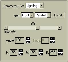
| The brain surface in the image above appears dark. This is because a) it is a semi-transparent surface, and b) the lighting is not optimal for this view. The lighting model(s) used can greatly influence the appearance of rendered 3D objects. Select "Parameters For: .. Lighting" and set the menu as indicated to the right. Selecting "From .. Flat" provides brighter light-sources that can tend to make some objects look flatter.
There are 3 distinct light-sources:
|
 |
There are 4 types of lighting models available to each of these sources:
The default is to have an ambient source (Horizontal), a divergent source (Front), and a parallel source (Right). If the source is ambient, you can change the intensity, but the location has no concept. For some reason, the Divergent source type adds little light, and its direction setting seems to have little influence on the display.
You can change the intensity and direction of a Divergent, Parallel, or Spot light source, which are conceptually similar to a large flashlight. Each light source has a location relative to one of the primary axis. The Front and Right sources can be rotated around the edge of a 50-degree cone, the axis of which points at the object. The Horizontal light source rotates around a circle at the axial center of the object, so you can position the light source in front of, behind, etc. the object. The light-sources (should) only affect the appearance of volume-objects, not of lines or the slices on the back walls. The following descriptions apply to any non-ambient light source:
You can also change the color of each light source. The default is pure white, where red (R), green (G), and blue (B) all have maximal values of 255. Setting e.g. green to 0 yields a red+blue=purple light. Changes in lighting color may not be apparent if your objects are already colored, so use grey-colored objects for best results. For instance, if you have a purely red object, green and blue light will not illuminate it; only red light will have an effect. By playing with the colors, angles, and intensities of each of the lights you can see effects ranging from interesting through eerie. The image to the right was obtained with the following color settings:
|
 |
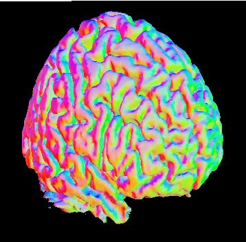 |
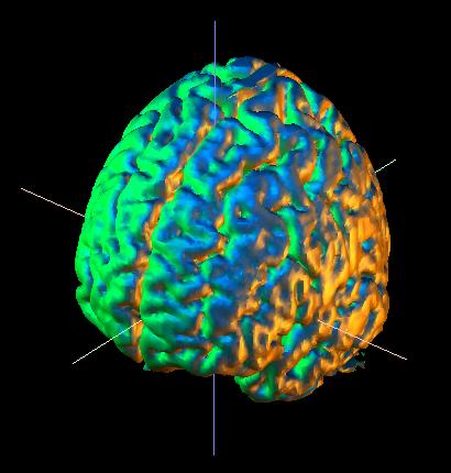
Yet another type of lighting effect can be obtained by shading the brain surface according to the orientation of the underlying elements of the mesh that constitute the basis for the rendered brain surface. From the "Parameters for: .. Surface" menu, click the "Directional Shading" box. This shades the object according to the direction of a normal line perpendicular to each small polygon in the brain surface's mesh.
Now go to the "Parameters for: .. Lighting" and set the "Right" and "Front" intensities to 0, and the "Horizontal" ambient intensity to 100 to get an image similar to that shown to the left. There is no exterior lighting source, but rather the brain has an inner glow of different colors coded according to the orientation of the surface mesh. Polygons with normal lines pointing toward the front will be green, toward the brain's right will be red, and toward the brain's left will be blue. It is important to note that this is not merely a lighting effect, as in the example above, but rather uses information from the brain surface in an informative way. This feature, while a bit gaudy, can be handy for emphasizing a particular sulcus or gyrus. |
Cuts within the brain: back to the Demo:
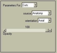 |
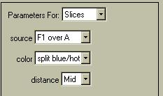
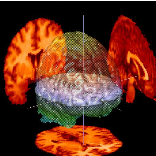
Now let's try to show a slice floating within the brain. Go to "Parameters For: .. Cuts" and set the menu up as shown to the left. You can select the volume you wish to display, and for each of the 3 orthogonal slices you can select an Opacity. If the Opacity is 0, the cut is not shown (or even created). You will get the best results if your images have been skull-stripped (as shown here), and/or if there is little information from outside of the brain surface (e.g. a [18F]-F-DOPA PET image).
You can combine up to three orthogonal cuts. The slice(s) at the current location will be displayed at their appropriate location within the image volume. You should now have an image resembling the following: |
| As you can see in the image like to the right, we are starting to fill up our proverbial 5-lb sack.
Let's get rid of the slices on the back walls, and change the brain surface color to "tissue". Go ahead, you can figure out how to do this on your own. |
 |
Anatomic Structures: ROIs etc.
Now, let's see how to show anatomic structures within the brain. For instance, ROIs drawn with SPAMALIZE's ROI drawing tool (BrainMaker) can be displayed as 3-dimensional objects. To take advantage of this feature, you will need to have a ROI mask volume drawn and saved from within BrainMaker. (Access the ROI tool by: "Analysis -> BrainMaker".)
Go to the "File: .. Mask" menu as shown below. Browse for the file ".../spamalize/data/nT1_ROImask.img". This is a ROI file that I created using BrainMaker, and it contains several somewhat hastily drawn anatomic structures.
![]()
A menu will appear as shown below. On some operating systems, this menu may appear and then get hidden behind one of the other SPAMALIZE menus (e.g. on Windows98). There will be one row for every structure within the ROI file that is recognized by BrainSpinner. Select a color for each of the structures you wish to display (as for the Caudate and Putamen below), and leave structures you don't want to see with a color "None". Then, you need to update the ROI mask volumes by Clicking the "Show Mask" button in the "File: .. Mask" menu as shown above. Voila! You should see your apparitionlike structures floating in the center of the brain.
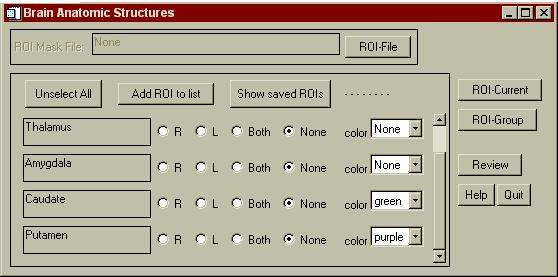
Warning! Do not select a color for "Whole Brain" here. You will be unable to see any other structures inside the brain. The brain surface is already displayed as the major "Surface" item if you have loaded in a skull-stripped MRI.
| You should now have an image that resembles the one to the right. The Caudate is shown in purple, and the Putamen is shown in green. These structures float in the middle of the brain, with their lower halves hidden by the (opaque) axial slice cutting through them. | 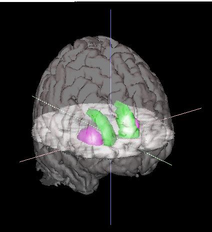 |
Activation Sites:
Now let's examine how to show a group of activation sites (e.g. from a SPM analysis) within the brain. Go to the "File: Functional 1" menu and browse for the file indicated in the menu below:

You can select any ANALYZE-formatted file you want, whether it comes from SPM or not. For instance, you could use functional PET or fMRI data. For the time being, however, let's assume you want to show SPM activations. In SPM99, you can simply select a con***.img, a beta***.img, or for the final results a spmF_***.img or spmT_***.img. The only caveat is that the functional image volume must be the same size (pixels) as the basis anatomy image volume.
For SPM96 results, you will need to ask me (Terry) how to use SPAMALIZE to convert the .mat result files to ANALYZE format. The file you selected above was created in this way from SPM96 results, and shows some generic blobs. Do not be alarmed that there are activations outside of the brain, I selected these data for that very reason.
 |
|
You have the same basic display options as for the Surface (source, style, color). Since these volumes are generally less complex than the Surface volume, the appearance does not revert from Smooth to Wire Mesh when you move the volume. For large or complex volumes, this means that movement will be slow...
You can select the level of smoothing at the bottom of the menu. Selecting "2" means that you are decreasing by a factor of approximately 23 = 8 times the number of vertices, which yields a smoother surface and faster movement. Smaller objects may be eliminated from view for higher smoothing values, and very small objects may be eliminated by smoothing values as low as 2.
If you want to show activation results from SPM99, you are in luck, because SPM99 now stores all of its results in SPAMALIZE-compatible format (i.e. ANALYZE files). If you want to examine a spmT_***.img, it likely has negative values in it so you need to account for this. The "show.. All" button on the right contains options to display "All" of the values, only the negative values ("Neg"), or only the positive values ("Pos").
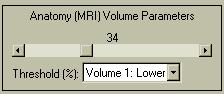 You can set the lower threshold in the Threshold menu, as shown to the left. This can be confusing because if you set the lower threshold below 0 and want to view "All" of the image, you are actually saying you want to see all of the 0-valued pixels surrounding the activation sites of interest, which translates as a large cube. To compensate, BrainSpinner automatically assumes that you want to see only the negative activations, and displays them. However, it can still be tricky to get the threshold set correctly, so you can explicitly state that you want to show either positive or negative values. In this case, the threshold value denotes the percentage of only the positive (or negative) values. If you have selected negative values, the lowest value (most negative) is treated as a high activation, and an activation cloud is built around these low values.
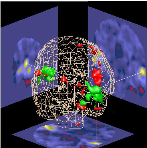 |
To show both positive and negative activations in different colors, you need to read the same volume into both the "Functional1" and "Functional2" volumes, then associciate "Volume1" with "Functional1", and "Volume2" with "Functional2". This usually takes a bit of experimenting, but can be quite useful, as shown in the image to the left.
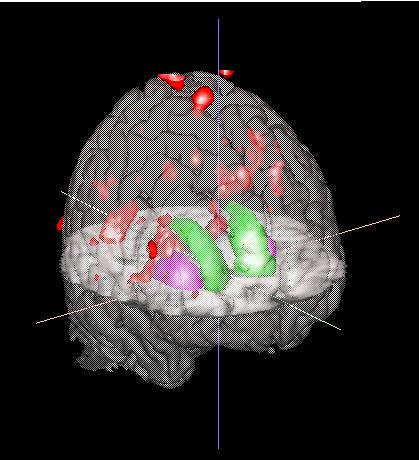
This image uses a SPM99-derived t-test parametric image different than what is used in the rest of this demo. The negative activations (in "Volume1") are shown in red, while the positive activations (in "Volume2") are shown in green. The images on the walls show the positive activations in yellow/green, and the negative acivations in red. (The spmT***.img activations are not overlaid on the anatomical images here, but rather are just displayed "as is" with the Stern color scale.) |
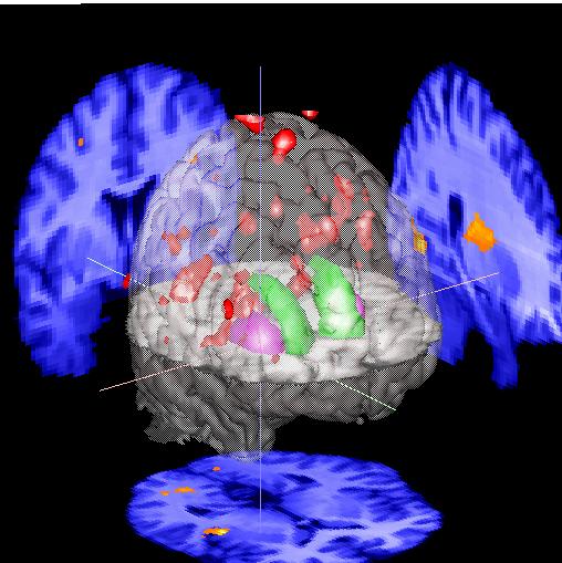
| You can show the activations displayed on the slices by going to the "Parameters for: .. Slices" menu, and selecting "source .. A, F". This causes the Anatomy volume to be displayed in blue, and the Functional volume is displayed in red. Where they overlap will be purple. | 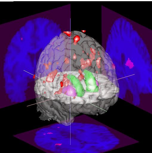 |
|
 |
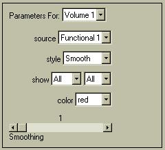
You can display 2 activation patterns simultaneously by reading the first activation volume into "Functional 1" and the second into "Functional 2". To display, select "Parameters for:..Volume 1", "source: .. Functional 1". Then repeat using "Parameters for:..Volume 2", "source: .. Functional 2". You might want to do this if you have a 2 different states or conditions, e.g. normal and diseased activation patterns, positive/negative correlation patterns, etc.
You can also show activation sites that are near the surface of the brain by color-coding them according to how far under the surface they are. Go to the "Parameters for... Surface" menu and select the appropiate volume you want to use for shading from the "Shading" menu. For instance, if you have a SPM analysis volume loaded into "Functional 1", select that. You can show deeper structures by increasing the "distance" parameter to a value greater than approximately 9 (mm).
Making Movies: The Cinema of the Mind.
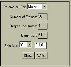 |
It is easy to make a MPG movie of a spinning brain. Select "Parameters for: .. Movie". The default parameters (shown in the menu to the left) are usually OK. Select "Show" to preview the movie, "Write" to write it to a file. You will get a more realistic movie by selecting more frames, but of course the .MPG file will be larger. The "Dimension" determines how many pixels wide and high the output movie will be. You can play with the Spin Axis settings to influence the axis about which the brain spins as well the amount of wobble. The idea is to spin about an axis which points along the normalized direction coordinates indicated. |
Changing your View:
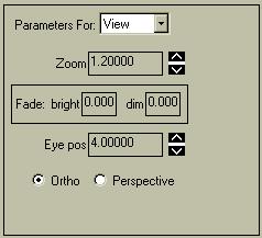 |
You can change several of the "global" aspects of the view from the "Parameters for ...View" menu. You can zoom in and out by changing the Zoom parameter. You cannot select a zoom value less than 1.2.
The "Fade: bright" and "Fade: dim" values let you control how the brightness of the objects changes with respect to position. The reference location is a plane parallel to the screen in the middle of the image volume; negative values denote planes closer to you, while positive values denote planes beyond the center. The actual values are in terms of "normalized" planes, where +/- 1.0 is a plane at the edge of the image volume.If the two values differ (i.e. both not 0.0) then all objects in front of the "bright" plane will have a normal intensity, all values behind the "dim" plane will be invisible (dark), and there will be a gradual fading of light to dark for objects between the two planes. You can have the object appear darker in the foreground by setting "dim" < "bright". |
The "Eye position" controls where an imaginary eye viewing the scene is located, in "normalized" coordinates. Here, positive values denote the eye position being farther from the image, which translates as closer to you. It can range from 0.1 - 10.0. If this value is less than 1.0, then portions of the object will be behind the eye and thus not viewed. This feature can help to see inside an object, but it can be frustrating to use for many objects. Results vary depending on whether you use "Ortho" or "Perspective" view.
The "Ortho / Perspective" radio buttons let you select an orthogonal view (the default) where orthogonal lines are shown as parallel, or a perspective view where parallel lines meet at some point way behind your monitor. The perspective view can be helpful in some zooming situations, as well as to take advantage of the "Eye pos" feature.
Writing Images:
![]()
You can write the currently displayed image to a .BMP or JPEG image using the menu above. These file formats can be put into most popular imaging/display programs (AdobePhotoshp, MSPowerpoint, MSWord, etc.). You can name the file something unique by typing in the text-box. Occassionally BrainSpinner gets confused and tries to reuse the previous name, which will over-write an existing file. Guard against this by typing a new name for each image. Ask Terry if you want another image format added- it is pretty easy to do.
Technical Details:
BrainSpinner uses all IDL object graphics. I don't recommend using this program on any computer slower than ~300 MHz. You will also need lots of memory (>128 MBytes).
If you happen to be using this on a MacIntosh, you may not have access to all of the features if you only have a single mouse button. You will need to figure out what combination of Cntrl buttons to press to mimic a second and third mouse button.
I made it so each of these objects can be added or removed from the view independently, and colors can be changed independently also. I don't use the IDLgrVolume, which I found too slow for interactive display. Instead, all of the rendered volumes are really IDLgrPolylines or IDLgrPolygons.