Picture Gallery

Features:
Picture Gallery
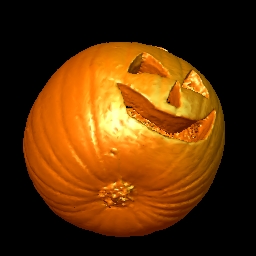
Seasonal Example. The images above were created by scanning a head-sized pumpkin in the MRI scanner (conversion from pumpkin to Jack-O-Lantern courtesy of Andy "Pygmaleon" Alexander). BrainSpinner was used to create a 3D rendering of the pumpkin's surface (inner and outer). Customized lighting was added to maximize the festive holiday mood. Finally, since we are after all in a brain imaging lab, we inserted a globe depicting the Earth's surface into Jack's cranium in the picture on the right.
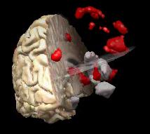
Example 1. The pictures above show two different views of a 3D rendered brain, with the right- and left-hand portion removed to reveal interior structures and activation areas. The posterior portion of the brain is closest to your vantage point. The structures(caudate, putamen, and amygdala) in the left-hand image are shown in grey, and in the right-hand image are shown in color (caudate=blue, putamen=green). Regions of the brain which were determined to produce an activation to an emotional stimulus in a large group of people are shown in red. These images took less than 5 minutes to compose and print, including fiddling around to get the perfect color of grey-brown for the brain surface.
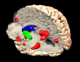
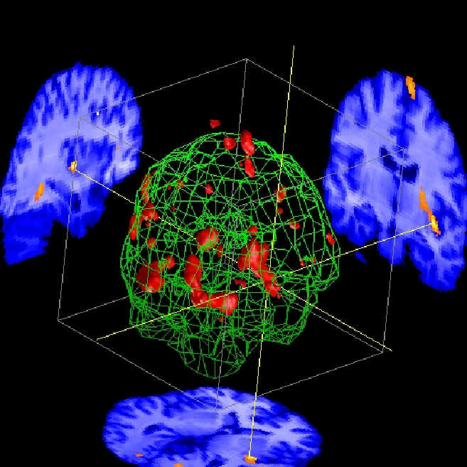
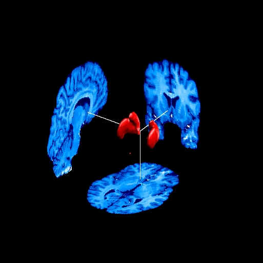
Example 2: Structure location. A MRI volume is displayed in the 3 orthogonal slices (axial, coronal, sagittal) on the back walls. The image on the right includes a semi-transparent outline of the brain (which probably has a funny appearance due to shrinking the image for display on this page). An activation area from a SPM analysis is shown as a red cloud, and is also shown as a yellow/red blob superimposed on the planar images. Several anatomic structures created as Volumes-of-Interest (VOIs) using BrainMaker are included as reference points for the SPM cloud: caudate (yellow), thalamus (green), amygdala (purple).
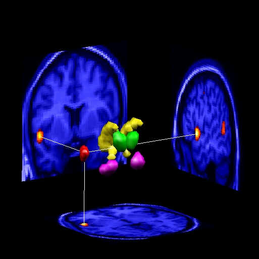
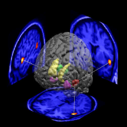
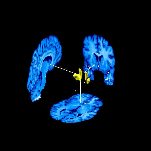
Example 3: Structure location. A MRI volume is displayed in the 3 orthogonal slices (axial, coronal, sagittal) on the back walls. Activation areas from a SPM analysis are shown asyellow/red blobs superimposed on the planar images, and also as numerous red clouds within the green wire-mesh outline of the brain. For spatially complex data with multiple locations and various shapes, this type of display is invaluable for showing the relative positions and extents of each activation. Clicking the mouse on any of the red clouds moves the current location (shown by the 3 orthogonal yellow lines) to that cloud, and updates the 3 back-wall images to show the corresponding slices at that location. Alternately, you can click on any of the 3 backwall images to move the current location to that point, updating the other two backwalls.
Example 4: ROI overlap. Two VOIs drawn by two different operators on the same hippocampus are compared as part of our inter-operator reliability testing. The above picture shows Operator #1's VOI in red and Operator #2's VOI in green. The two VOIs mostly overlap, but it is evident that Operator #1 (red) has included an anterior, superior region not included by Operator #2, while Operator #2 (green) has tended to include more tissue in the posterior, superior region. We have found this graphical representation to be immensely helpful in developing criteria for drawing ROIs and achieving good inter-operator reliability.
| Figure 4.1. F-DOPA PET scan (Normal) | Figure 4.2. F-DOPA PET scan (Parkinsonian) |
 |
 |
Example 5: Functional Regions. Both pictures above show three orthogonal views of a PET scan taken with the tracer [18F]-F-L-DOPA, which is accumulated in dopaminergically active regions of the brain, such as the caudate and putamen. The left-hand figure (4.1) shows a scan of a normal, healthy person. The PET scan was thresholded to create the green clouds, which show the functional extent of the cuadate and putamen. The right-hand figure (4.2) shows a scan of a Parkinsonian subject. This PET scan was thresholded similarly to the normal PET scan, and the markedly reduced functional extent of the caudate and putamen become evident.
| Figure 4.3. Functional Striatum (Normal elderly) | Figure 4.4. Functional Striatum (Parkinsonian) |
 |
 |
The anatomical extents (visible with MRI) are generally similar for normal and Parkinsonian subjects. The pictures above show a different pair of normal (fig. 4.3) and Parkinsonian (Fig. 4.4) subjects than in Figs. 4.1 and 4.2. The functional volumes shown by the [18F]-F-L-DOPA tracer have been delineated similarly, only here the volumes are shown relative to a MRI scan (one MRI scan used to demonstrate relative position for both subjects).
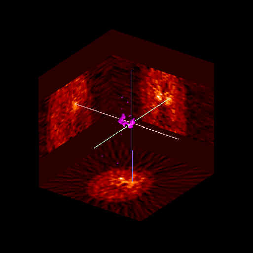
Example 6: PET Phantom Display. The above picture shows a "phantom" scanned in a PET scanner. A phantom provides a known geometry and activity concentration and is used for scanner testing and diagnostics. This particular phantom was a tub filled with a modest amount of radioactivity to simulate a typical cerebral FDG scan. The warm background contained various sized spheres filled with a radioactive solution that was either twice the concentration of teh warm background (hot-spots, near or left side of phantom), or half the concentration of the warm background (cool-spots, far or right side of phantom).
The planar views show the pattern of warm background and hot- and cool-spots, for the location indicated by the purple lines. The central 3D rendering shows the various spheres color-coded according to their diameter: red=22mm, green=17mm, yellow=9mm, blue=4.7mm. The rendering of the warm background (the tub) shows the back side of the tub as a solid wall, and the front side of the tub is a mesh.
So- you can give that long explanation, or just show the picture... As with all of the other views shown on this page, this rendering can be rotated in real time using the mouse as a virtual joystick.
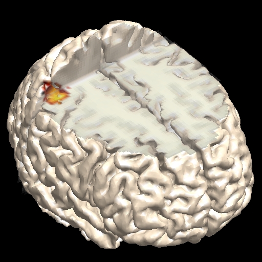
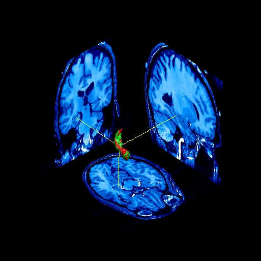
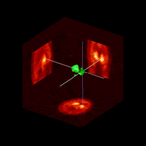
Example 7: SPM Activation Location. The red-orange spot shows an SPM activation location. The color of the spot is related to the level or intensity of the activation (yellow shows the most intense activation, in the center of the spot). A portion of the brain has been removed to reveal the interior anatomic structure.
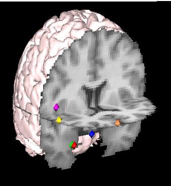
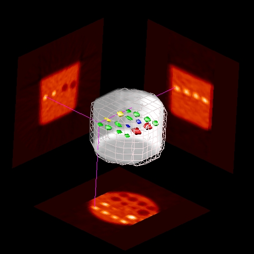
Example 8: Activation Locations Culled from Literature Findings. The picture above shows six (6) different activation areas for various cognitive preocesses, as reported by six different authors. (The locations are not supposed to match up.) BrainMaker was used to create small ROIs denoting the location of each of the six author's findings in Talairach coordinates. The ROIs were then shown in BrainSpinner as 6 different-colored blobs, with each blob corresponding to a different author. A coronal and an axial slice are shown to help orient the blobs and to provide some idea of the relative distances from the brain surface, while the surface of the brain posterior to the anterior commisure is shown to give a sense of the overall proportion.