Table of Contents:
Multiple-time graphical analysis (MTGA) is a technique used to quantitate PET and SPECT data that involve a radioactive tracer studied over time as it accumulates in a tissue region. Typically, the data are acquired as a series of dynamic frames, beginning with tracer injection and continuing until either the radioactive decay severely limits the statistical content of the images, or until the acquisition disk fills up!
The fundamental assumption is that the tracer accumulates in a specific anatomic region. If it continues to accumulate "forever", so there is never a net egress of tracer from the tissue, then it is known as an ireversibly bound tracer and a Patlak-plot is appropriate. If the tracer accumulates for some time and then washes out, it is a reversibly bound tracer and a Logan plot is more appropriate.
The input data required for MTGA include a dynamic series of tomographic data (PET or SPECT images) and an input function or time-activity curve (TAC) of the tracer concentration in the blood. This is a very general technique, and has been used for many neurotransmitters ([18F]-F-DOPA, [18F]-FMT, [11C]-raclopride, etc.), metabolism markers ([18F]-FDG), and even for cardiac applications.
The underlying goal of this type of graphical analysis is to reduce a series of observations to a single value that can be compared across subjects. Since the tracer concentration in tissue changes over time for most PET tracers, a single high-statistic image is not appropriate. On the other hand, an image acquired over a short time period where the change in tracer concentration is minimal will have relatively poor signal:noise qualities. Thus, various graphical approaches were developed to use short time frames with acceptable temporal resolution, yet effectively use all of the events counted over an extended period of time.
Model-based Alternative Approach:
An alternative to the graphical analysis approach is a model-based approach, e.g. the 3-compartment FDG model. In this approach, a series of compartments are posited into which the tracer can flow. The flow into the first compartment(s) is governed by an input function, which is the tracer concentration measured in blood (or perhaps in respired air). Flow into and out of other compartments is governed by rate constants. The observed data (PET images) are generally fit to the model. Depending on the model, the input function can be used either as a type of scaling factor, as in the FDG model where the rate constants are assigned an a priori value, or as a dynamic factor in estimating rate constants.
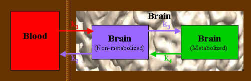
One problem with a model-based approach is that you need at least one observation for every parameter you are trying to fit. In a 3-compartment model, there are 4 parameters: transport from blood into tissue (k1) and back (k2), and transport from a tissue non-metabolized compartment to a metabolized state (k3) and back (k4), as shown below.
Thus, at least 4 seperate observations or frames are required. As the model becomes more complicated, more observations are needed; splitting a given acquisition time into shorter frame lengths means that the image quality of each frame is degraded. Some help can be obtained by fixing some of the better-known or less important parameters as constant values, and a wealth of valuable information can be obtained using a model-based approach. However, this approach is limited by noisy data and the need for enough observations to fit the model at hand. Frequently the data are noisy enough so that even with many more observations than parameters, the data cannot support the desired model complexity.
The graphical method was originally developed to address the relatively simple case where a tracer is irreversibly trapped in tissue. In reality, very few tracers are truly trapped forever as there is almost always a metabolic or physical path out of the tissue. A tracer is considered irreversibly trapped if no efflux is noticed during the length of the PET scan. For this case, a so-called Patlak plot was developed. (Albert Gjedde first proposed this approach in 1981, but Patlak's seminal 1983 paper in which he formally developed this method caused his name to be associated with it.)
A Patlak-plot is not model-specific. This means that, although a model can be ascribed to the underlying system for the purpose of interpreting the results, there is no a priori requirement for a particular set of compartments. An arbitrary series of compartments can be diagrammed as follows:
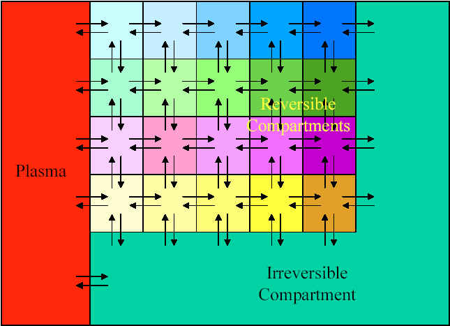
Any of the Reversible compartmants can be grouped together into a single compartment. As long as the system can be modeled so that the flow out of the Irreversible compartment is negligible, then this is an appropriate case for a Patlak-plot analysis. Another way of saying this is that the rate constants governing egress from the Irreversible compartment are individually and together negligibly small.
A Patlak-plot involves creating an ordinate and an abscissa using various combinations of the input function and image data at each of the observed time points:
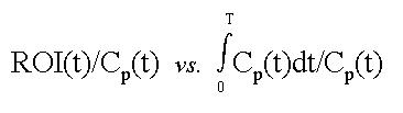
where ROI is the concentration of a tracer in a tissue region-of-interest, t is the elapsed time from injection to a particular frame, and Cp is the concetration of tracer in plasma.
There is one observed time-point for every PET frame. This time-point is assigned to the center of the PET frame. A time-activity curve (TAC) is obtained for a particular region-of-interest (ROI), and the value of the ROI at each frame has a corresponding time-point. The ROI value represents the overall concentration of radioactivity in the tissue (which is not necessarily the same as the tracer concentration). A TAC for the input function (Cp(t), the concentration of tracer in the plasma) is created by interpolating the measured plasma curve to the middle of each frame. For every frame, a the ratio of the ROI value in that frame divided by the plasma concentration is plotted as a function of the integral of the plasma curve (from t=0 to the current time) divided by the plasma concentration at that time-point.
The first thing to notice about this plot is the units. The dependent variable is unitless, since both the ROI and the plasma values have units of concentration: microCi/ml. The independent variable has units of time (seconds), since the other units cancel out. The second thing to notice is that both the abscissa and the ordinate are divided by the same thing, namely Cp(t). This method can be thought of as a way of scaling the the tracer concentration in a region of tissue by the opportunity the tissue had to absorb the tracer over time.
So far this doesn't seem very helpful. However, it was noticed that such a plot becomes linear at those time-points when the transport of tracer into the trapped compartment is essentially unidirectional. Patlak showed that the slope of a line fit through this linear region is equivalent to the influx constant, Ki, for the system. Ki can be defined as the ratio of the total amount of tracer accumulated in a tissue region after an infinite amount of time, divided by the integral of the plasma TAC from t=0 to infinity.
In his 1985 paper, Patlak went on to show that two of the assumptions in his earlier work could be relaxed:
The first point is important because it is difficult to find a tracer that has absolutely no egress from a compartment.
The second point is important because it is frequently difficult to obtain an adequate blood TAC. Furthermore, if a tracer is metabolized, it is even more difficult to separate the tracer concentration from the overall blood concentration of radioactivity. Using a reference region obviates the need to measure the blood TAC and separate the various metabolites. It is important to note that results using a measured blood input function cannot be directly compared with results using a reference region.
Jean Logan et al. developed a graphical method to explicitly deal with reversibly bound tracers, which have a net efflux constant that is non-negligible compared to the influx constant. Her approach involves creating a plot with the following axis:
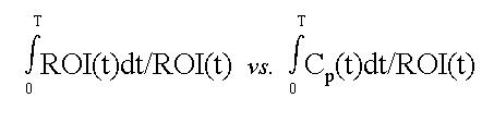
where (as in the Patlak equation) ROI is the concentration of a tracer in a tissue region-of-interest, t is the elapsed time from injection to a particular frame, and Cp is the concetration of tracer in plasma. The Logan-plot still divides both abscissa and ordinate by the same value, but here the divisor is ROI(t) as opposed to Cp(t) as in a Patlak-plot. Also, the ROI(t) term in the ordinate is integrated with respect to time.
Like the Patlak-plot, the slope and intercept of a Logan-plot have distinct interpretations depending on the actual model you choose to ascribe to the underlying system. The line in a Logan-plot should be fit through those frames that are linear; these frames usually occur somewhere in the middle of the plot. This is another way of saying that data should be collected long enough to see a net efflux of tracer from the region of interest.
The following papers are all excellent. They provide a nice explanation of the theory behind the MTGA approach as well as explain a particular implementation. Jean Logan's 1986 paper summarizes earlier work and is my pick for a starting point.
Gjedde A, "High- and low-affinity transport of D-glucose from blood to brain", J. Neurochem., 36:1463:1471, 1981.
Logan J, Fowler JS, Volkow ND, Wang G-J, Ding Y-S, Alexoff DL, "Distribution volume ratios without blood sampling from graphical analysis of PET data", J. Cereb. Blood Flow Metab., 16:834-840, 1986.
Logan J, Fowler JS, Volkow ND, Wolf AP, Dewey SL, Schlyer D, MacGregor RR, Hitzemann R, Bendrium B, Gatley SJ, Christman D, "Graphical analysis of reversible radioligand binding from time-activity measurements applied to [N-11C-methyl]-(-)-cocaine PET studies in human subjects", J. Cereb. Blood Flow Metab., 10:740-747, 1990.
Logan J, Volkow N, Fowler J, Wang G, Dewey S, MacGregor R, Schlyer D, Gatley S, Pappas N, King P, "Effects of blood flow on 11C-raclopride binding in the brain: Model simulations and kinetic analysis of PET data", J. Cereb. Blood Flow Metab., 14:995-1010, 1995.
Patlak CS, Blasberg RG, Fenstermacher JD, "Graphical evaluation of blood-to-brain transfer constants from multiple-time uptake data", J. Cereb. Blood Flow Metab., 3:1-7, 1983.
Patlak CS and Blasberg RG, "Graphical evaluation of blood-to-brain transfer constants from multiple-time uptake data. Generalizations", J. Cereb. Blood Flow Metab., 5:584-590, 1985.
MTGA GUI Tool Introduction.
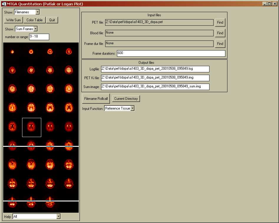
The MTGA Tool is part of the Spamalize suite of tools. It is named "spw_mtga.pro", and represents ~5000 lines of IDL code. Access the tool from Spamalize's main menu via "Analysis -> Patlak Plot". A menu will appear that resembles the one shown below in the "File Menu" section. There are actually several different menu screens within this menu. The left-hand menu is always visible, while the content of the right-hand menu changes to show the various stages of creating a Patlak/Logan plot. The various screens are accessed by selecting an item from the "Show" menu in the upper left corner.
An alternative non-GUI VOI-based MTGA tool is available. This program lets you draw VOIs using BrainMaker, then automatically calculate Patlak/Logan plots for every VOI in the group.
The left-hand menu is always visible. It contains general control items. The most important item is the "Show..." dropdown menu. It lets you navigate from one menu to another in the right-hand display. See the example in the "File Menu" section below. Options include:
The items in the dropdown menu are arranged in the order you must address them in a standard analysis. However, a handy thing about the dropdown menu is that you do not have to visit every menu. For instance, if you are reading in a blood file, you can skip right to the MTGA Plot menu. The TAC menu will still be displayed, but it will quickly be replaced by the MTGA plots menu. Underneath, the program is set up so it can figure out what data it needs to process in order to be ready for a desired menu. If for some reason a piece of data is missing, you will not be allowed to visit the menu(s) where you would use that data. Instead, you wll be returned (usually) to the File menu. I'm sure you can figure out a way to trick this aspect of the program, but so far I have not.
"Write Sum" lets you write a sum-image of the currently selected frames to a 3D ANALYZE file. This is useful if you want to draw ROIs using another program such as BrainMaker.
"Color Table" allows you to select a color table for your image display. It is important that you use the "Color Table" button in the MTGA Tool, and NOT another button from a different Spamalize module (such as in the Spamalize main menu). If you load a color table using a different tool, the ROI display and line colors will get all messed up.
"Quit" will, as the name suggests, quit out of the application. When you restart MTGA Tool, you will start with a clean slate. This is nice if you genuinely want to start fresh, but can be annoying if you have to reload all of your old data.
"Show: Sum Frames" is a dropdown menu that affects what gets displayed in the raw PET window in the left-hand menu. The default is to show a series of sum-images, for data summed over several frames. Other options include "Frame", to display a single frame, and "Plane", to sum images over several planes within each frame. (The latter is generally a bad idea but is included for completeness.)
"number or range" lets you select which Frame, Plane, or range of summed frames to show. This is a clever entry box that does its best to figure out what you want. If you want a single frame, type a number like "10". If you want a range of frames, type something like "8 - 10" (inclusive). You will not be allowed to enter frame values outside of the loaded range. Make sure to hit "Return" when you are finished editing this text box! After hitting "Return", the new Frame/Plane/Sum-image will be displayed.
When the tool opens, the "File" menu (shown below) is active. (The image display and file text-boxes will be blank until you actually load a dynamic series of images.)
Load Image Data:
To load a file, click the "Find" button to the right of the "PET file" text-box. Browse for a file and select "OK" from the browser menu. The file will take approximately 5-10 seconds to load. You are not allowed to access any other menu items or move to another menu until you have loaded a dynamic PET data set. Currently, you can load either a GE/Advance PET file, or a 4D ANALYZE file. When the image data are finished loading, a sum-image of the latest frames will be displayed in the bottom part of the left-hand menu, as shown above.
Frame Durations:
If you load a GE/Advance file, all of the timing information for the frames is in the file's header section, and gets automatically loaded and processed. If you load a 4D ANALYZE file, you need to supply the frame durations (in seconds) for each frame. You can do this by typing the frame info into the "Frame durations" text box. An example might be:
60 60 60 60 120 120 120 600 600 600 600 600 600 600 600
which would span a typical 90-minute F-DOPA protocol. Notice how the frame durations are shorter in the beginning, to bettter capture the time-course of the tracer, while longer frames at the end provide better statistics. You could also type this sequence into a text-file and save the file, then load the file by clicking the "Find" button to the right of the "Frame dur file" text-box. If you load in a GE/Advance file, you can also override the frame information by typing your own values into the "Frame duration" text-box, although this is normally not a good idea.
Blood TAC:
The other piece of data you need to create a Patlak/Logan plot is some knowledge of the opportunity the tissue had to take up the tracer. This is expressed as an "input function", also known as a time-activity curve (TAC) of the concentration of the tracer in the blood. There actually two options here:
There is an in-depth discussion of these options in the next section, "Tissue Reference Menu". For now, let's just see how to load in a blood TAC file. Click on the "Find" button next to the "Blood file" text-box. Browse for a blood file. (See the section "TAC File Example" for more details on file format.) You may select any text-file with a valid TAC. Spamalize can also automatically read a TAC file if you follow a particular naming convention: put the file in the same directory as the image data, and name it with the same prefix as the image data but with the suffix "_blood.txt". For example, if your image data file is named "a1234_fdopa.pet", call your blood file "a1234_fdopa_blood.txt". The file will then be automatically loaded into the MTGA Tool. You may, of course, load a new file in if you like, but this feature is handy if you will repeat the analysis of a particular image file several times.
Output Filenames:
When you read an image file, a series of potential output filenames are created, shown in the "Output files" section of the file menu. When you actually write a particular piece of data, the corresponding filename will be used. You may redirect output data to a different file by editing the appropriate text-box. Generally, the MTGA Tool will do everything it can to avoid overwriting an existing file, so you don't need to worry about renaming your output files every time you turn around. The renaming feature is included in case you don't care for the conventions selected by Spamalize.
The tissue reference menu lets you define a ROI for a reference region. This is not necessary if you already have loaded a blood TAC file. However, you may wish to use a reference region in conjunction with a blood TAC in order to subtract the reference region from your Patlak/Logan ROI, in order to use the MTGA intercept as an estimate of e.g. the distribution volume from a Patlak plot.
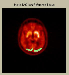 To draw a reference ROI, simply depress the left mouse button and draw your ROI. Releasing the mouse button closes the ROI. Use the right mouse button to draw an "inverse" ROI, i.e. to delete part or all of an existing ROI. Click on one of the images in the "Raw PET" menu on the left to show that particular image in the Draw-ROI window. The selected image will have a white box drawn around it. The reference ROI will be displayed in green, as in the picture below of a ROI over the occiptal cortex.
You may draw on several planes to define a 3-dimensional "volume-of-interest". All ROI voxels will be included in the reference ROI, regardless of which plane they are in. All ROI voxels are weighted equally.
You can also read in a ROI that you drew using another program (e.g. BrainMaker) that permits greater accuracy. Select the "Read Mask" button and browse for the file. It should be a 3D file that is coregistered to the 3D framewise PET data. The image dimensions (X,Y,Z) must match. The desired tissue reference region must have non-zero values, and all other (background) pixles must be set to zero. To compare results from this program with another, you may write out the tissue reference mask by clicking on the "Write Mask" button. A mask file will be written to an ANALYZE-7.5 format file.
When you have drawn or imported a reference ROI on at least one plane, you may move on to the TAC menu.
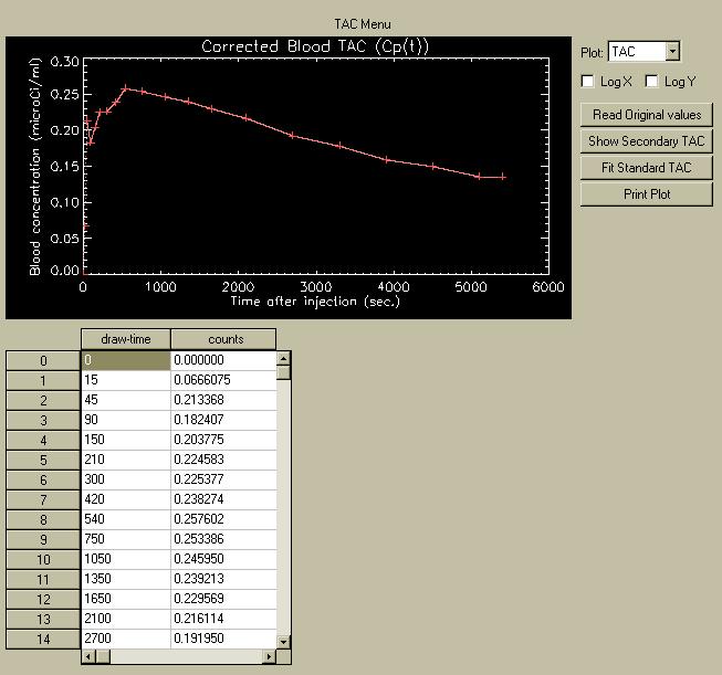
The TAC menu displays and allows you to edit the time-activity curve (TAC) that is your input function. Getting a likable TAC is a challenging part of the data collection scheme, so the MTGA Tool gives you a few options to examine your TAC and to see the effect small (or large) differences have on your results. Normally you should get your TAC "perfect" before entering the MTGA Tool. However, life and especially that part of it devoted to science is rarely perfect, so the TAC menu lets you play "what if".
For instance, "what if" my patient's blood line didn't clog during the first 3 minutes, and I was able to measure the entire input function? Well, you can change the first point you DID measure so the integral of the TAC is similar to what it would be if there was a nice high peak at 40 seconds, and then see how the new TAC affects your results. Similarly, you can read in a complete (good) data set, and examine the effect of removing the peak. Occasionally, you may get to the TAC menu and notice from the plot that one of your points is out of whack. Rather than edit the blood file and load it back in, you can simply edit that point, and set it to something that makes sense.
The TAC menu shows a plot of the TAC, and also contains a table showing the draw-times and tracer concentration for each sample.
To edit the values in the TAC, double click on the value, edit it, then hit "Return". A new plot will be drawn showing the change. You may change as many points as you wish. However, you cannot add new points without loading a new TAC file. You can change the times, but only so the new time is still between both of its original neighbors. When you leave the TAC menu and move to the MTGA Plot or Image menu, the current values in the table get written to the log-file, so whatever changes you made can be reproduced later.
The TAC always runs from 0 seconds through the end of the last frame. If you do not have a zero (0) point, a time-point will be inserted automatically into the TAC with zero (0) counts. Similarly, if you do not have measured time points to the end of the last frame, a new time-point will be appended with the last value you do have. These points are added to ensure that the interpolation scheme (used to extract the TAC value at a particular time) functions properly.
The table shows at most 15 TAC points. To see more (if there are more), use the scroll bar on the right side of the table. It is worth noting that eventually ALL of the TAC measurements get interpolated to create a set of points for the middle of each PET time-frame. If you want to compare the MTGA tool results with another program, it is important that all comparisons are performed using the middle of the time frames as the standard.
A TAC file should be a simple ASCII text file with 2 columns. The first column should contain the time (in seconds) after radiotracer injection when a particular blood sample was drawn from the subject. The second column should contain the decay-corrected concentration of the tracer. Note that this is frequently not the same as the overall concentration of radioactivity in the blood! If the tracer is metabolized by the body (and most are) a fraction of the radioactivity in the blood will be due to the metabolites. Some tracers, such as [18F]-F-DOPA, have a number of metabolites and there is a complex relation between the actual tracer concentration and the overall radioactivity concentration in the blood. Precise and technically difficult measurement of the tracer concentration is required to obtain an adequate tracer TAC in such cases.
The TAC file should resemble the following example, which contains nothing else except a time (in seconds) relative to injection, a decay-corrected concentration of tracer, and a "Return" character on each line:
0 0.000000
15 0.0666075
45 0.213368
90 0.182407
150 0.203775
210 0.224583
300 0.225377
420 0.238274
540 0.257602
750 0.253386
1050 0.245950
1350 0.239213
1650 0.229569
2100 0.216114
2700 0.191950
3300 0.177779
3900 0.158761
4500 0.149534
5100 0.135415
5400 0.135415
This is an example from a reference TAC that was written to a log-file. I used it to avoid typing a lot of numbers in. I mention this because there will be two differences for a typical measured blood TAC:
TAC Menu Options:
"Log X" and "Log Y" allow you to display the X- and/or Y-axis of the plot on a logarithmic scale, which is handy if there is a large range of values.
"Read original values" reads the original values from the blood file, in case you got headed too far down the change lane.
"Show secondary TAC" lets you superimpose a TAC from a different TAC file on top of the original TAC. This lets you compare TACs from different subjects, or from the same subject on different occasions.
"Fit Standard TAC" is not yet implemented, but eventually it will fit whatever sparse TAC points you have to a population-average TAC and yield a subject-specific input function. Watch this space.
"Print Plot" allows you to send the current plot to a printer. For non-UW sites this requires special configuration of Spamalize. (Well, it does here too, but most people don't have to worry about it.)
When you get a TAC you like, whether it is from a measured blood source or from a reference region, you are ready to create a Patlak or Logan plot.
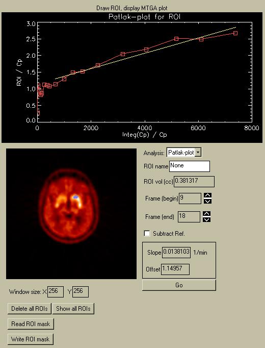
The MTGA plot menu lets you create a Patlak- or Logan-plot using a dynamic image series and an input function TAC. When you enter the menu, the plot region will be empty. After you define a ROI and click "Go", the menu will resemble the picture below:
Defining a ROI.
To draw a ROI, follow the same procedure as for the Reference region. Depress the left mouse button to draw a ROI. Release the mouse button to close it. Use the right mouse button to draw an "inverse" ROI, i.e. to delete part or all of an existing ROI. Click on one of the images in the "Raw PET" menu on the left to show a particular image in the Draw-ROI window. The selected image will have a white box drawn around it. The ROI will be displayed in blue, as in the picture below of a ROI over the right caudate. Also, the ROI will be displayed in blue over the raw PET images in the Control Menu (see below).
Instead of drawing a ROI in the MTGA Plot menu with the concise but limited ROI drawing tool, you may instead elect to draw the ROI in a full-fledged ROI drawing tool like BrainMaker, and then read the ROI into the MTGA Tool. The ROI that you create must be stored as an ANALYZE-formatted file. The X,Y,Z-dimensions must be the same as for a single 3D frame from your original image data. Click "Read ROI mask", and browse for the ROI file. All non-zero values are used to create a 3-dimensional ROI mask. Any previously drawn ROI will be deleted and replaced with the new ROI, and the display will be automatically updated to show the new ROI.
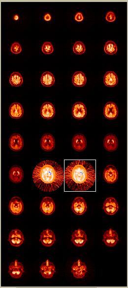 "Show all ROIs" updates the display of ROIs on the raw PET images, as shown in the picture to the left. The ROIs are shown in blue over the striatum (caudate + putamen) of two of the central images in this example. The color-table becomes altered slightly to enhance the background of images containing part of an ROI. This facilitates seeing the planes you have drawn on, which can be difficult for very small ROIs.
"Delete all ROIs" clears all voxels from the current ROI, allowing you to draw a fresh ROI. This is handy if you have drawn a ROI over several planes. It can be tricky to find all of the small ROIs in every plane, so clicking this button ensures that you are indeed starting anew.
"Write ROI mask" lets you write a 3D ANALYZE file containing a bit-mask (0s and 1s). This is handy if you want to compare this MTGA Tool to another one. By writing the mask, you can then use the tool of your choice to extract the time-activity curve of the ROI from the PET data and perform the Patlak/Logan analysis in a spreadsheet. (You can also do this using the data printed to the MTGA Tool's logfile, but writing the maks provides independent confirmation that all is well.)
You can change the window size if you like: simply enter the width you desire (pixels) into the "Window size: X" text-box. The Y-size is linked to the X-size, so changing the X-size will also change the Y-size. If you want a different Y-size, you can enter the desired value after you change the X-size. Make sure to hit "Return" to cause the changes to take effect! Usually a 400x400 window is large enough to provide good control over drawing a ROI using the MTGA Tool's drawing facility.
You may select either a Patlak-plot or a Logan-plot analysis using the "Analysis" dropdown menu. Both analysis require the same basic input, so you can select either option for any data set, but the interpretation of the results depends on the tracer. See the theory section for when one approach is more appropriate than the other. Clicking "Go" will run whatever analysis type appears in the "Analysis" dropdown menu.
When you draw a ROI , you may wish to name it. Fred, Ginger, amygdala, whatever. Every time you click "Go", a new analysis is performed and the new results are written to the log-file. Using a particular ROI name will help you keep track of what you did when you review the log-file. You can enter a string of (almost) any length. Make sure to hit "Return" when you are done editing!
The ROI volume is displayed in the "ROI vol (cc)" text-box. The volume is in cubic centimeters (ml). It applies to the entire volume-of-interest, not to a single plane. Its accuracy depends on knowing the volume of the voxels in the image data. For GE/Advance data this is usually accurate, but for 4D ANALYZE image data you must ensure that the header values are correct.
The primary result of a Patlak- or Logan-analysis is expressed as the slope of a line fit through a portion of the Patlak- or Logan-plot. See the theory portion for more information about this. The slope and offset of this line appear in the box at the lower right of the menu. You may select which frames to use for the line fit via the "Frame begin" and "Frame end" text boxes. (Remember to hit "Return".)
You may elect to subtract the Reference-tissue values from the corresponding ROI values by checking the "Subtract Ref" box. (See the theory section on when this might be appropriate.)
As mentioned above, every time you click "Go" and perform an analysis, the results get written to the log-file. A single log-file is used for each image file session. The name of the file is displayed in the "Filename" menu. Summary information is written, such as the Patlak (Logan) slope and offset and the the ROI voume. Also written are values from each frame, such as the ROI averages, blood TAC values, etc. Using the information written to the blood file, you can verify that the program is working as intended.
A key feature to note is that all times are referenced from the middle of every time-frame. This is the time-point most representative of the PET/SPECT data in that frame. For blood TAC values, the original TAC is interpolated to the middle of each frame. The various integrals are summed from t=0 to the middle of the frame of interest. Bear this in mind when comparing to another program!
You can create a parametric image for every plane, showing the voxel-by-voxel slope for a line fit independently through the time-series for each voxel. The values obtained from this approach are different (generally smaller) than values obtained from a ROI approach. Smoothing the images helps slightly, but the utility of these images should be considered mainly for display purposes, and also for investigating potentially fruitful areas to perform a ROI analysis.
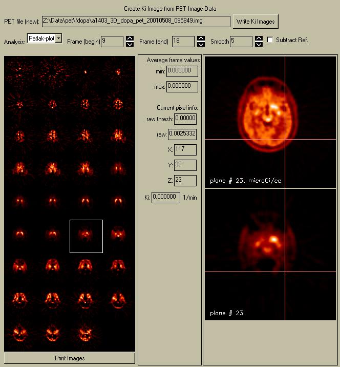
When you enter this menu, the parametric images are automatically calculated and displayed. It takes ~5 seconds to calculate a new set of parametric images (faster than reading the data in!). The new influx or so-called "Ki" images are displayed in a window that appears next to the original PET images. These display images are not scaled to a common global maximum, but rather each image is scaled to its own global maximum. Otherwise, only a few of the images in this example (those containing the caudate and putamen) would have any visible regions. You can click on either the images in the raw PET menu or the Ki image display to select and display a new plane in the zoomed image windows on the right-hand side of the menu.
The data values at any point can be seen by moving the cursor over either the raw PET image (top) or the Ki image (bottom). The raw PET value under the cursor appears in the "raw:" textbox, and the Patlak/Logan value appears in the "Ki" textbox. The current location (1-based) appears in the "X", "Y", and "Z" textboxes. Clicking with the mouse in the images shows a pink crosshair, so you can compare locations between the two images.
Similar values for analysis type, frame-span, and "subtract ref" appear in this menu as in the MTGA plot menu. These values are actually linked, so changing e.g. the "Frame (begin)" value in this menu will also change the same value in the MTGA Plot menu.
The data generally need to be spatially smoothed in order to have a desireable appearance. You can experiment with different smoothness levels with the "Smooth" parameter. A square smoothing kernal is centered on each voxel within each plane and the average mean is taken of the pixels inside the kernal. This is sometimes called a 2D boxcar-type mean.
Both Patlak- and Logan-plot images are supported. These images can be considered quantitative, as the slope calculated for any single voxel with no smoothing is the same as the slope calculated using a ROI for that voxel. However, you should not compare results obtained for different levels of smoothing.
You can write the Ki images to a 3D ANALYZE file by clicking "Write Ki images". The data will be written to the filename shown to the left of this button. You can send the Ki images to a printer by clicking the "Print Images" button.
References:
Gjedde A, "High- and Low-affinity transport of D-glucose from blood to brain", J. Neurochem, 36:1463-1471, 1981.
Logan J, Fowler JS, Volkow ND, Wang G-J, Ding Y-S, Alexoff DL, "Distribution volume ratios without blood sampling from graphical analysis of PET data", J Cereb Blood Flow Metab", 16:834-840, 1986.
Logan J, Fowler JS, Volkow ND, Wolf AP, Dewey SL, Schlyer D, MacGregor RR, Hitzemann R, Bendrium B, Gatley SJ, Christman D, "Graphical analysis of reversible radioligand binding from time-activity measurements applied to [N-11C-methyl]-(-)-cocaine PET studies in human subjects", J. Cereb. Blood Flow Metab., 10:740-747, 1990.
Logan J, Volkow N, Fowler J, Wang G, Dewey S, MacGregor R, Schlyer D, Gatley S, Pappas N, King P, "Effects of blood flow on 11C-raclopride binding in the brain: Model simulations and kinetic analysis of PET data", J. Cereb. Blood Flow Metab., 14:995-1010, 1995.
Patlak CS, Blasberg RG, Fenstermacher JD, "Graphical evaluation of blood-to-brain transfer constants from multiple-time uptake data", J. Cereb. Blood FLow Metab., 3:1-7, 1983.
Patlak CS, Blasberg RG, "Graphical evaluation of blood-to-brain transfer constants from multiple-time uptake data. Generalizations", J. Cereb. Blood FLow Metab., 5:584-590, 1985