This page demonstrates an analysis of a simple fMRI visual stimulation experiment, using two different approaches:
The data and analysis steps can be found at:
/study/training/spm99/visual_stim/data
/study/training/spm99/visual_stim/SPM_anal
While in the MRI scanner, the subject was shown an alternating series of either a blank screen (baseline) or pictures of faces (activation condition). The face stimulation will affect both the visual cortex in general, and the face-processing regions of the brain such as the Fusiform Gyrus (FG).
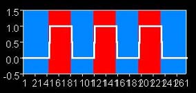
There were a total of 110 acquisitions or fMRI frames. (There were actually more, but a few extra images at the beginning and end of the run were removed from the current working data set.) The presentaion sequence was as follows:
Frame # Condition
------- ---------
1-10 off
11-20 on
21-30 off
31-40 on
41-50 off
51-60 on
61-70 off
71-80 on
81-90 off
91-100 on
101-110 off
This presentation scheme yields a robust signal in the visual cortex (posterior or back of the brain). We typically detect this signal by knowing the presentation scheme, and performing a correlation of the model of the presentation function with the time course of each voxel. The model in this case is a boxcar function, represented by 0's and 1's:
000000000011111111110000000000...11111111110000000000
or graphically like the following (but with 2 more red/blue pairs):
If you are the Keck Lab, the data set can be found at:
/scratch/fMRI_data/data
Here you will find the original data, and data sets for each of the pre-processing steps (motion correction, spatial normalization, and smoothing). There are also two similar analysis performed. You can work through the entire analysis, or just cut to the chase and examine the results displayed below.
Before we plunge into a complicated correlational analysis, lets first try a simple subtraction approach. We simply sum all of the image frames from the baseline condition, then sum all of the image frames from the stimulation condition. The two sum-images are converted to average-images, in order to put the values on the same scale as the original data. Then, we subtract the baseline image from the stimulation image to (hopefully) reveal the activation locations.
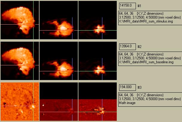
Figure 1. The top row shows the stimulation sum-image, the middle row shows the baseline sum-image, and the bottom row shows the difference images. Left column:sagittal, center column: axial (anterior on left side of image, left side of brain at bottom of image), right column: coronal (top of brain on left side of image)
The subtraction image shows a small activation in the region of the visual cortex, which is what we expect. There is a similar activation on the right-hand side (show below). The magnitude of the activation is 1.3%. There are several other areas that appear to be activated as well. For instance, in the bottom center picture, the white spot at the left shows a large difference (23%), but this is centered over the right eye and is most likely an artifact related to movement. However, there are a few bright (and dim) spots in the subtraction image that are plausibly within the brain. The problem is to figure out which spots are true acti\vations, and which ones are due to an artifact or noise.
The first step is to create a mask of the brain, so that only voxels which are actually in the brain are examined. This can be done by selecting a threshold and excluding all voxels with a value below that threshold. These data range from 0 - ~25000; a threshold of 7000 was used for the following image:
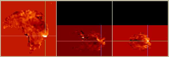
Figure 2. Masked difference image (stimulus - baseline).
The contrast has improved, since regions such as the eyes with small values but a large difference are no longer considered. However, we still don't know which of the remaining hot-spots (or cold-spots) to believe. A reasonable starting point is to determine which voxels have the most believable values, and to weight those voxels more than others. A common way to assess the certainty with which a value is known is to calculate its variance. So, the variance across all voxels from the baseline condition was calculated, and the masked activation image was divided by the variance image. After some further thresholding to remove areas with unusually high variance, we arrive at the following:
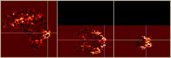
Figure 3. Masked difference images, weighted by the variance in the time series for each voxel.
The region shown in Figure 2 is no longer very bright, so we can conclude that this area has a lot of variance, and the hot-spot shown in Figure 2 is not very trustworthy. Several other regions have now become more dominant. This difference image is much noisier than the previous one, and we are (or should be) left wondering, really, how much we can trust these results.
If you jumped right away to this section, you probably already know about SPM. If not, SPM (Statistical Parameteric Mapping) is an approach, embodied in a program called SPM99, which attempts to tell us not only the location and relative magnitude of activations, but also tries to ascribe a statistically valid certainty to discovered activations. (There are several other widely-used programs that act similarly; links to some are here.)
In the following discussion, items in red type indicate non-SPM programs, and items in blue type indicate SPM-related menu items that you select or enter.
I. These data were converted from AFNI format with the following commands:
A. convert data to axial format:
/home/oakes/progs/AFNI/3daxialize -prefix a -orient LPI ./run_2_volreg+orig.BRIK
Note use of "-orient LPI", which is how the SPM templates are oriented.
If your data were acquired sagittaly with the left slice first (left-to-right), then you need to substitute "RPI" in the above command to yield a radiologically oriented image. The assumption in the Keck lab is that all MRI data have a radiological orientation prior to input into SPM. (You should check your data to assure this.)
B. Convert data to SPM99 (ANALYZE) format:
/home/oakes/progs/AFNI/3dAFNItoANALYZE fMRI_vis_stim/scratch/fMRI_data/data/a+orig.BRIK
The raw data look like this:
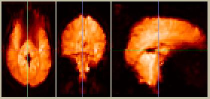
Figure 4. Raw data from frame 10, in the default SPM orientation. The images in Figures 1-3 were not reoriented from their sagittal acquisition.
II. Pre-processing:
Start SPM, go to "fMRI" side.
A. Slice Timing Correction:
It is a good idea to perform slice-timing correction, but it is somewhere between tricky and painful to do this in SPM if your data were not acquired axially. Hint: don't try to use the "Reorient images" button in SPM99. It updates the .mat files but not the image files. However, it appears that the slice timing correction module is not smart enough to apply the .mat files to the data prior to performing the STC, so it gets it all botched up... I would suggest using AFNI to do STC, then export the data to ANALYZE format for compatibility with SPM.
B. Motion Correction:
Realign (~10 minutes to calculate transforms and then reslice images)
Number of subjects: 1
Num sessions for subject 1: 1
[Select files, all 110 of them]
Reslice interpolation method: sync
Adjust sampling errors? no
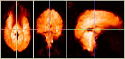
Figure 5. Motion-corrected data, frame 10. These images look very similar to the pre-motion-corrected data in Figure 4, since movement is typically on the order of 1 mm or less.
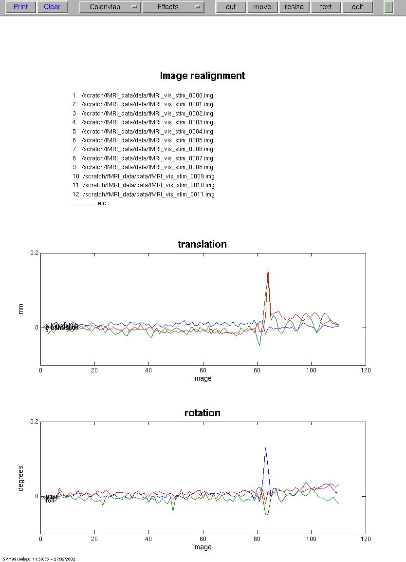
Figure 6. SPM99 screen after motion-correction. THe parameters show the estimates for translation (mm) in the X-, Y-, and Z-dimensions, and rotation (degrees) avout the X-, Y-, and Z-axis. Note the relatively large spike at about frame 82. Interestingly, these data were already motion-corrected by AFNI. Visual inspection of the raw data shows a distinct movement between frames, as if the subject sneezed or swallowed. Inspection of the motion-corrected by either AFNI or subseuently SPM99 shows a similar (but smaller) motion, indicating that the movement probably occured during a frame, and the data have actually become corrupted.
C. Spatial Normalization:
Spatial normalization is the process of transforming an image volume into a known coordinate system. In this case, we used an average brain developed by the Montreal Neurological Institute (MNI). The main reason to spatially normalize brain images is so that one individual's data can be combined with other subjects from a group. Since we are not combining our example with other subjects, we don't really need to spatially normalize it, but after all this is a tutorial so we'll do it for the sake of thoroughness.
Normalize (~10 minutes to calculate one transform and reslice all images)
Image to determine parameters from: meanfMRI_vis_stim_0000.img
Images to write normalized: rfMRI...0-109.img (all realigned images)
Template image(s): EPI_template_mommri.img
(This is a template developed at the Keck Lab which uses a number of scans from our scanner)
Interpolation method: Bilinear
At this point the data have been coregistered to the MNI template, and interpolated to 2x2x2mm voxels:
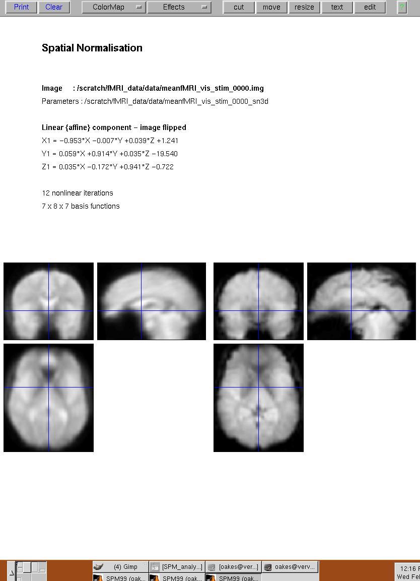
Figure 7. SPM99 screen after spatial normalization. The template image is in the left, the spatially normalized average-image (created during motion correction) is on the right.
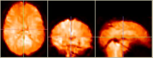
Figure 8. Spatially normalized data, in the MNI reference frame and converted to 2x2x2mm voxels.
D. Smoothing:
Smooth (~8 minutes)
smoothing {FWHM in mm} 8 8 12
select scans: [select the 110 nornalized scans:]
The smoothed data look, well, smoother:
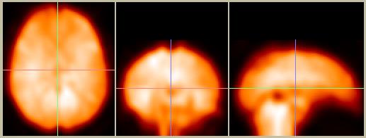
Figure 9. Smoothed and spatially normalized data (compare to Figure 8).
III. Set up the SPM model:
fMRI models (~2 minutes to set up model, ~4 minutes to run it)
What would you like to do? specify and estimate a model
number of sessions: 1
select scans for session 1: [select all of the 110 smoothed scans]
interscan interval {secs} 3
number of conditions or trials: 1 [N.B.: Baseline doesn't count!]
name for condition 1? visual stim
SOA: fixed
SOA (scans) for visual stim: 20 [10+10]
time to 1st trial (scans): 10
parametric modulation: none
are these trials: epochs
Select type of response: fixed response (boxcar)
convolve with hrf: yes
add temporal derivatives: no
epoch length {scans} for visual stim:10
interactions among trials (Volterra): no
user specified regressors: 0
remove Global effects: none
high-pass filter? specify
session cutoff period (secs): 126
Low-pass filter? hrf
Model intrinsic correlstations? none
Setup trial-specific F-contrasts? yes
estimate? now
Your model design should look like the following:
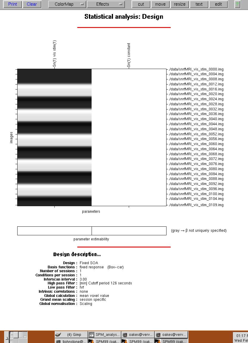
Figure 10. SPM99 screen showing statistical model. The boxcar function is shown from top to bottom in the collumn of alternating dark (baseline) and light (stimulus) conditions. A hemodynamic response function was convolved with the boxcar function, yielding the blurred edges.
IV. Results
Select the "SPM.mat" file from you analysis directory
F-contrasts: Session 1: vis stim
mask with other contrasts? no
title for comparison: Session1: vis stim
corrected height threshold: yes
corrected p value: 0.05
The glass-brain view appears.
Click on button "volume" to see summary
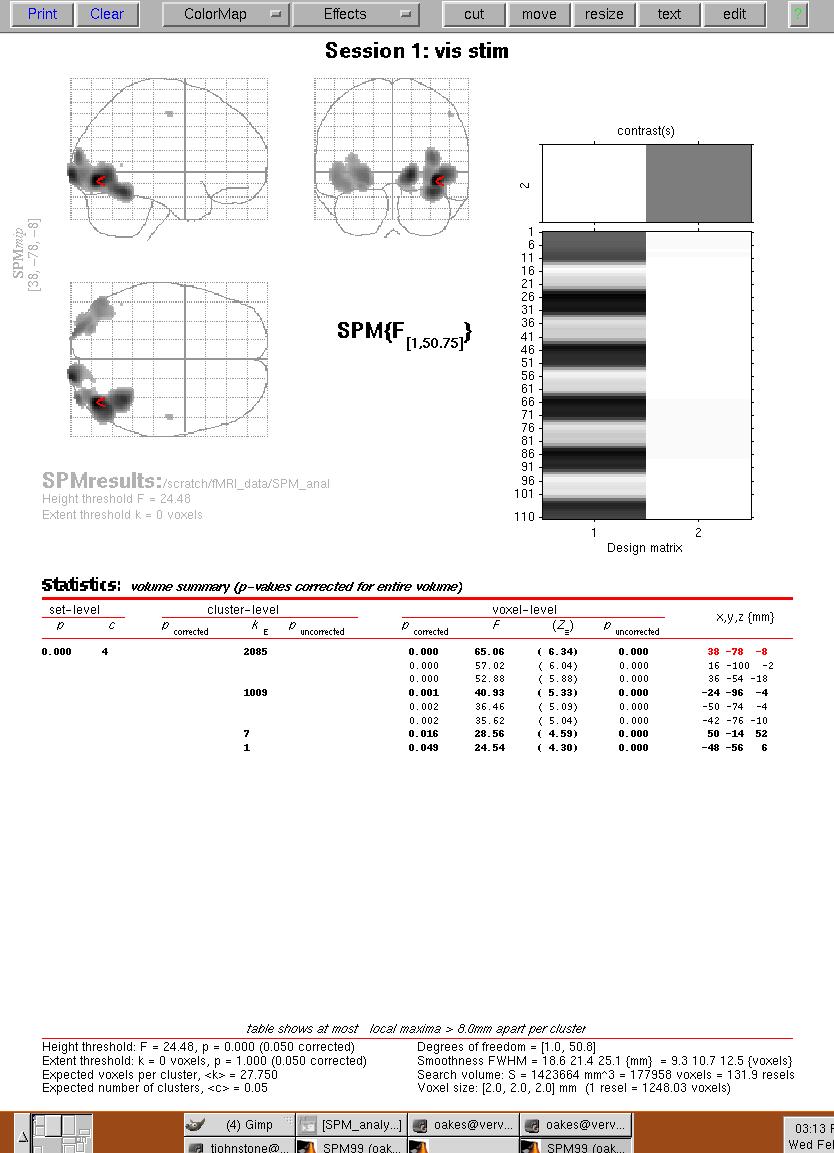
Figure 11. Results menu from SPM99 menu. The "glass brain" view is shown on the top, and a summary of the major clusters is displayed at the bottom. The red arrow shows the location of the largest F-value for the largest cluster. You can click on a cluster location (under the "x,y,z (mm)" column on the bottom right) to move the red triangle to that location.
You can look at the time-course of any voxel by clicking on the "Plot" button on the menu on the lower left panel.
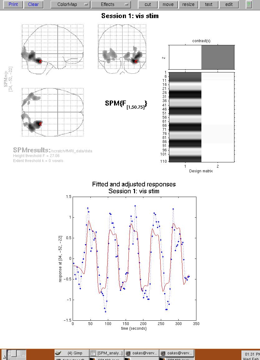
Figure 12. Plots of fitted and adjusted responses for a single voxel (where the red triangle is located).
Now click on the button "overlays -> sections", and select the T1 template image from SPM99's template directory. The activation results above the selected threshold will be shown as follows:
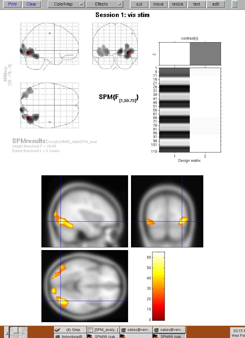
Figure 13. Activation results overlaid on average T1-weighted template image. The cursor is centered on a region that includes the Fusiform Gyrus.
So by this time you may be wondering why the activation location is not exactly the same as in the subtraction experiment. Well, it depends on what type of activation you want to examine... SPM99 produces a series of intermediate images leading up to the final output shown in Figures 10-13. These images include:
1) beta_***.img: these are created during the estimation stage - i.e. the fitting of the model. There is one beta image per column of the design matrix. These are the parameter estimates of course, with the first ones corresponding to the variables of interest, the last one corresponding to the constant in the model.
2) con_***.img: these are created when calculating t-contrasts and correspond to weighted sums of the beta weights. The numbering of the contrast images corresponds to the number of the contrast created in the contrast manager
3) SPM{t} is computed by dividing the contrast image (con_***.img) by its standard error (a multiple of the square root of ResMS.img). The SPM{t} is saved as spmT_***.img.
4) ess_***.img: these are images of the extra sum of squares for the corresponding F-contrasts, corresponding to the con_*** images from a t-test..
5) SPM{F} is essentially an extra-sum-of squares test (See Draper & Smith "Applied Regression Analysis"), where the additional variance explained by a section of the model is compared with the error variance. In other words, the F-test is concerned with how much a given variable *uniquely* adds to explained variance. SPM{F} is spmF_***.img, computed by dividing the ess_***.img by the ResMS.img error variance estimate image, and scaling appropriately.
The t-contrast basically tells us about whether a specific linear contrast of beta estimates differs from zero. The F-contrast tells us about how much a given linear contrast of parameter estimates (as a subset of such contrasts) contributes uniquely to explaining variance in the data.
The Beta-images show a voxel-by-voxel map of the parameter estimates required to fit each voxel's timecourse to the boxcar model. In this case there are two parameters, a global parameter and a parameter for the difference between conditions.. These two Beta-images look like this:
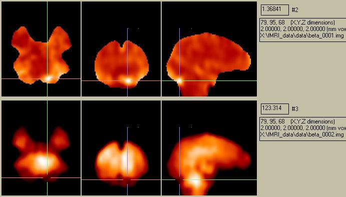
Figure 14. Beta-images showing voxel maps of parameter fits.
The map of Beta001 looks remarkably similar to the map shown in Figure 2 of the subtraction analysis. The goodness-of-fit estimate map (calculated as the residual error) looks like this:
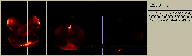
Figure 15. Residual error map.
Note that the residual error map (Fig. 15) shows a high error (i.e. more uncertainty) in the region of activation picked out by both the subtraction image and the Beta1 image. Since we only created an "SPM{F}" image (showing ALL effects of interest), the ess***.img corresponds to the con***.img for a SPM{t}image.
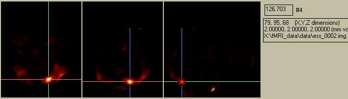
Figure 16. The weighted beta image for the effect of interest.
Dividing ess_0002.img by the ResMS.img yields the following:
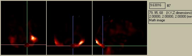
Figure 17. A simple ration image (calculated outside of SPM99) of the ess*.img divided by the ResMS.img.
which has a pattern that is remarkably similar to the SPM{F} image which SPM99 spits out:
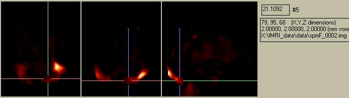
Figure 18. The SPM{F} image, showing a summary of the locations and statistical certainty (but not necessarily the magnitude) of differences between the baseline and activation condition. Note that there are other considerations in SPM99, so the magnitude of the simple ratio image is not the same as the SPM{F} image.
It is important to realize that the final SPM{F} image does NOT necessarily show regions with strong activations, but rather regions where we are SURE there was an activation. This is where the "Statistical Parameter" part of "SPM" comes into play: we are mapping a parameter that indicates the statistical certainty of an activation, not the activation magnitude. In the preceding example, the strongest activation (i.e. the region in the visual cortex with the largest baseline/stimulation difference) is also relatively noisy, so we cannot be too sure about how reliable it is. On the other hand, the activation in the Fusiform Gyrus is relatively small, but is quite consistent.
Interestingly, the Fusiform Gyrus has been shown by many researchers to be related to facial processing.