This page prvides instructions for how we apply SPM's Slice Timing Correction to our data in the LfAN. There are two anomolies in our fMRI data that make this recipe non-standard:
STC Recipe:
This recipe is based on the "momMRI" data set. Your directory organization may be somewhat different.
1) Go to the directory where your original reconstructed files live. Slice-timing should be performed before realignment, smoothing, or anything else. This directory will be referred to as
/.../orig/
2) If there are any *.mat files in this directory, make a new directory named /.../orig/mat_files and move them into it (or better yet delete them- you should be starting fresh).
3) Rotate all of the image volumes into a coronal orientation. When you are done, the front (anterior) of the brain should be the first coronal slice. The instructions below refer to options from the indicated Spamalize menu (or later, from the SPM menu).
4) Move coronal images into a new directory, /.../orig/cor/
5) Use SPM's Slice Timing Correction module.
I suggest writing this array in a text-editor, and copying and pasting it into the text-box. This should help avoid errors.
6) Move all of the slice-time-corrected files into a new directory.
7) Flip all of the slice-time-corrected data back to an axial orientation, ready for input to SPM99. This is the same sequence of events as flipping the original images into the coronal orientation, only you want to use a different suffix, and select the opposite direction for rotation.
8) Move the axial STC data into a new directory:
These images are now ready for input to SPM99 for Realignment (aka motion-correction). If you want, you can delete all of the intermediate files once you are satisfied that you have succesfully followed this recipe. How will you know if it is right? You can compare the pre- and post-STC images in Spamalize.
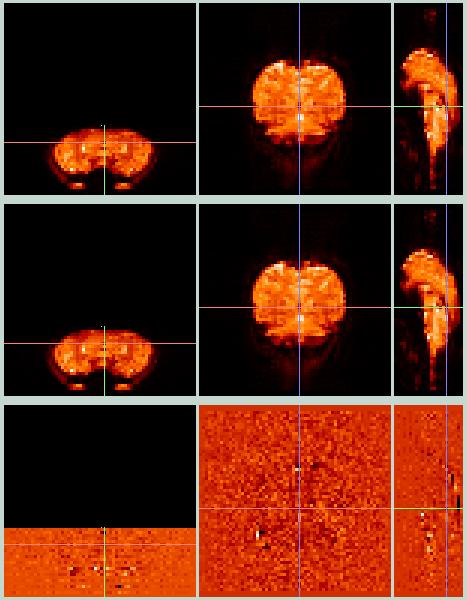
The pre image is in the top row, the post image in the middle row, and the difference image is in the bottom row. From left to right, the axial, coronal, and sagittal views are shown. It should look something like:
The main thing to notice is the axial (and sagittal) difference image. See how in the anterior part of the brain (bottom of axial view), where there is the least correction, the difference image is the smoothest? Toward the posterior part (top of axial view), the image is much noisier, indicating larger corrections in both the positive and negative directions. Also notice how the interleaving pattern is evident in the axial and sagittal difference images.
The average correction in these images was on the order of 2-3% or less, although there are (disturbingly) a very few pixels that changed by more than 50%! These latter pixels tend to be right at the edge of the brain, over a blood vessel or both. Bear in mind that the magnitude of the BOLD signal changes we are looking for is 1%-2% (or less!) so this can be a significant alteration to your data.