Help for SPAMALIZE's FDG Quantitation Tool
last updated on: August 28 2001.
Outline
of FDG Help:
A. Basics
B. Interface
C. Run It!
A.
Overview
B.
PET data
C.
Blood data
D.
Ideal blood curve
E.
Model parameters
F.
Blood file example
A. Filenames
B. Blood TAC
C. Kinetic Model
D. Metabolic Images
A. Overview
B. Printing data
C. Log file
A.
Basics
SPAMALIZE's FDG quantitation tool (SPW_FDG.PRO) converts raw [18F]-FDG PET data
to metabolic rate images. These are called "quantitated" or
"metabolic" images in the vernacular, and are commonly used to
compare the local cerebral metabolic rate of glucose consumption (lCMRglu)
between different subjects, or between the same subject scanned on different
occasions.
This program
implements a variation of the Sokoloff method as presented in Phelp's landmark
1979 paper:
Phelps
ME, Huang SC, Hoffman EJ, Selin C, Sokoloff L, Kuhl DE,
"Tomographic measurement of
local cerebral glucose metabolic
rate
in humans with (F-18)2-fluoro-2-deoxy-D-glucose:
Validation
of method", Ann Neurol 6:371-388, 1979.
There are 3
main parts in this program:
1) Create a
time-activity curve (TAC) from measured blood data;
2) Calculate
the correction factors to convert PET data from units of radioactivity
concentration to metabolic rate.
3) Apply the
correction factors to the PET data.
This program is designed to read GE/Advance PET data. Formats from other scanners could be easily incorporated with a bit of programming. Intermediate results can be saved and applied to other analysis if desired. The default behavior is to run through in one fell swoop. This program has been tested (successfully!) on SUN/unix and PC/Windows98 and PC/Linux platforms.
This program
was written by Terry Oakes in December 1999 at the Lab for Affective
Neuroscience in the Psychology Department, University of Wisconsin-Madison.
Information in this help file supercedes any other information. Examples of the
GUI interface can be found on the SPAMALIZE website:
http://psyphz.psych.wisc.edu/~oakes/spam/spam_frames.htm
B.
Interface Overview
There are 5
distinct menus in this program.
1) Main control and raw image display. This menu is on the left-hand side of the GUI and is always visible. The original (raw) PET images are displayed here, and there are also a few buttons for moving through the other 4 menus. Pressing the "Write Log" button will cause a log-file to be written containing the current parameters and status. There is a Blood-File viewer available through this menu as well, so you can plot blood files without having to load in a PET data set. For an example of the menus, see the "Filenames" section below.
Only one (1)
of the other four (4) menus is visible at a time. These 4 "Action"
menus can be seen in the right-hand side, and are accessed by the dropdown menu "Show" at the top of the
left-hand menu.
The Action
menus are:
2) Filenames: Shows required input filenames, lets user browse for and load files, and lets user override default names
for output files. This is the menu which
is visible when you begin.
3) Blood TAC: Display and manipulate measured blood data.
4) FDG Model: Displays the FDG model and its parameters, and allows you to see the effect on typical data values.
5) Metabolic Images: Displays metabolic images and average values.
Moving
between any of the four Action menus causes the appropriate values to be
calculated. For instance, moving from the Filenames to the Blood TAC menu
causes the blood data to be read in and a new TAC is created. Moving from the
Filename to the Metabolic Images menu causes all of the intermediate steps to
be run, i.e. a new TAC is created, the FDG model is run, and finally the
metabolic images are created and displayed.
C.
Run It!
It is simple
to create a set of metabolic images using SPW_FDG. If your data are in the
default locations and in the expected formats, you only need to do three (3)
things:
1) Browse for
a GE/Advance raw PET file;
2) Move to
the Metabolic Images menu;
3) Select the
"Write Metabolic Images" button.
That's it!
You will automatically progress through the Blood TAC and the FDG Model menus. It is wise to stop at each of these menus to examine your input data, but this is not required. If there are any problems, it is most likely due to problems with the blood file.
A.
Overview
Several files are required by SPW_FDG. Two of these files are the raw PET data and the blood file you are interested in. The other files are standard files that are the same for every analysis and are stored in SPAMALIZE's data directory.
Explicitly,
the four (4) required data files are:
1) 18F-FDG
PET scan, currently from a GE/Advance PET scanner;
2) Blood file, in the format defined elsewhere in this help document;
3) Population-average blood TAC on a 1-second grid (several variations);
4) Kinetic
model parameter file.
B.
PET data
This program uses data from the GE/Advance PET scanner. Other file formats could be used with some modification (see comments in program). The data should be the result of a "IEE Unarchive" operation. At the Keck Lab, Robert Pyzalski or Terry Oakes usually do this.
Previous protocols (prior to 1999) named GE/Advance PET files something like:
a1234.mac128
where:
- 1234 is the
patient scan number
- mac stands
for "measured attenuation correction", the alternative is
cac, which stands for "calculated
attenuation correction".
- 128 is the
size of the reconstructed images, i.e. 128x128 pixels.
Current protocols (1999 and later) should use a naming convention like:
a1234_mac128.pet
In their native format, GE/Advance images are stored with the top of the head in plane #1, with the anterior portion (nose) stored first in each image, and in the radiological convention (patient's left appears on the right-hand side of the image). If the images are displayed by starting to draw from the bottom of a window (which is the default for SPAMALIZE, IDL, and many image display programs) the images will appear upside-down. This program (SPW_FDG) begins drawing from the top, so the images will appear right-side up. However, there is no flipping of any
The GE/Advance data can include a single frame or multi-frame data. The standard approach used by GEMS in creating a PET file is to decay-correct each image to the scan_start, which is the time of the beginning of the scan (not necessarily the frame). The program used to read the GE/Advance data (SPAM_READ_GE) spits out images that have all corrections applied and are in units of radioactivity concentration (microCi/cc). During the course of quantitation, the PET data get further decay-corrected back to the time of injection, so that the PET data are comparable to the blood data. For this reason, it is imperative that the blood file be accurate.
C.
Blood data
The blood data should be in an ASCII text file, in a format defined elsewhere in this Help document. Typically the blood data are named something like:
a1234_blood.txt or a1234
where "1234" is the scan number of the corresponding PET scan. (The simple "a1234" convention is obsolete.)
The blood data are needed as the link between how much radioactivity is measured in each brain pixel, and the opportunity that each brain pixel had to store that radioactivity. In general, brain regions that store
Typically we
measure as fast as possible for the first 2 minutes (1sample/10 sec), then 1
sample/30 sec for 2 min, then 1 sample/min out to 10 min, then 1 sample/5 min
out to 30 minutes. The whole blood is spun in a centrifuge, and 0.5 ml of
plasma is drawn off and counted in a gamma- (or well-) counter.
Usually the
gamma-counter decay-corrects the counts to the injection time using the program
"halflife", but occasionally this does not happen. The
decay-correction attempts to remove the effect of radioactive decay from the
detected counts, i.e. the goal is to "normalize" the counts so that
it does not matter how long after injection the samples were actually counted.
If the "Decay_corrected" field in the blood file is "yes",
this means the samples have all been decay-corrected to the indicated
"Injection_time", using the appropriate half-life (109 min) and
branching ratio (0.97) for 18F positron decay. If the "Decay_corrected" field is "no", SPAMALIZE will perform the decay correction using the elapsed time from injection to the time when each sample was counted. If SPAMALIZE performs the decay-correction, you need to make absolutely sure that the gamma counter did not already try to do this automatically. During the course of quantitation, the PET data get decay-corrected back to the time of injection, so that the PET data are comparable to the blood data. For this reason, it is imperative that the injection time listed in the blood file be accurate.
The data from
the well-counter are reported as "counts per minute" (CPM). The
samples are usually counted for 30 seconds, but nevertheless since the counts
are reported as CPM, the count duration entered into the blood file should be 60 seconds.
There is a blood-file plotter available from the Control Menu. You may plot up to 40 different blood files. After pressing the "Blood Tool" button in the Control Menu, the Blood Tool will pop up:
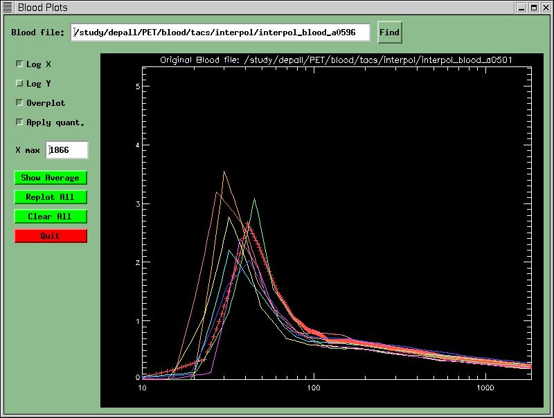
You may plot up to 40 blood files with this tool for comparison. It is currently a bit crude, in that it scales all subsequent plots to the first one until you press "Replot All'. In addition to reading the text blood-files, this tool can also read in blood data stored as a 1-sec gridded TAC. See the population-averaged blood TACs for an example of this.
D. Population-averaged blood curve
Most people have a blood time-activity curve (TAC) with a similar and reproducible SHAPE (not value) after approximately 20-30 minutes. Also, most (>50%) of the FDG uptake has already occurred by 30 minutes, so the subsequent values are only marginally important to the overall computed lCMRglu. We take advantage of this by only sampling blood out to 30 minutes, and then using a composite TAC (created from ~6 normal subjects) for the time from 30 minutes to the end of the PET scan.
The population-average curve we use extends out to 2 hr, 10 min (or, 7800 seconds). If you have acquired PET data which extends beyond this time, you cannot use this curve.
At the Keck Lab, the file is stored in:
/apps/spamalize/data/fdg_avg_bloodcurve.txt (unix)
or
W:\apps\spamalize\data\fdg_avg_bloodcurve.txt (Windows)
At the Brogden Lab, the file is stored in:
/local/progs/spamalize/data/fdg_avg_bloodcurve.txt (unix)
or
W:\local\progs\spamalize\data\fdg_avg_bloodcurve.txt (Windows)
If you are elsewhere, look in your SPAMALIZE installation directory:
/.../spamalize/data/fdg_avg_bloodcurve.txt
The population-average curve gets scaled to the measured curve in order to make a smooth transition after the last measured blood point. If your last measured point looks like an outlier, you might want to consider changing it to create a reasonably smooth blood curve. The population-average curve has also been scaled to allow quantitation without any blood curve, using only the injected does, body weight and perhaps the height. These scaled files are discussed below.
E.
Model parameters
The model
parameters are simply the rate constants (k1-k4) and the Lump Constant (LC)
that describe the kinetics of the FDG model, as given in [Phelps, 1979]. There
are actually different values appropriate for different tissue types (i.e. gray
and white matter). However, we do not know ahead of time which tissue
corresponds to a given pixel. Since we are primarily interested in the gray
matter values, we use the rate constants for gray matter throughout the entire
brain.
The file
containing the rate constants and Lump Constant is stored in:
/.../spamalize/data/fdg_model_params.txt
Following is an example of a blood file. It should be a simple ASCII text file. Some header-type information is at the top, with a title and value on each line. There is one row per blood sample. Comments appear in [square brackets]; do not include the brackets or what they contain in the blood file. If "Decay_corrected" is "yes", this means the samples have all been decay-corrected to the indicated "Injection_time", using the appropriate half-life (109 min) and branching ratio (0.97) for 18F positron decay. If decay-correction has been performed properly, including running the "halflife" program, the values in the fourth column (measurement time) should all be the same. They are different in the example below.
The headings for each column are: number, draw-time, measurement time, counts, counting duration (seconds), and sample volume (ml). The values in the first column (number) MUST start at 1 and increments of 1. If you missed a sample, do NOT indicate this by omitting its designated sample number. Also, the injection time MUST be the same as or earlier than the first blood sample time.
The text
between the dotted lines is a sample file:
-------------------------------------------------------------------
Ecat_calibration_factor
1
Decay_corrected yes [or "no"]
Glucose_1 102
Glucose_2 108
Glucose_3 107
Counter_type gamma
Dose 5.2 [mCi]
Patient_mass 240 [lbs.]
Patient_height 170 [cm]
Injection_time 11.33.02 [hh.mm.ss]
1 11.33.08 12.44.16 18.3 60 0.5
2 11.33.19 12.45.10 0.0 60 0.5
3 11.33.28 12.45.52 30122.3 60 0.5
4 11.33.38 12.46.40 791403.5 60 0.5
5 11.33.48 12.47.28 590763.5 60 0.5
6 11.33.58 12.48.16 331228.0 60 0.5
7 11.34.09 12.48.58 279327.2 60 0.5
8 11.34.20 12.49.46 204265.8 60 0.5
9 11.34.52 12.50.34 145213.6 60 0.5
10 11.35.30 12.51.22 151695.6 60 0.5
11 11.36.01 12.52.04 150084.4 60 0.5
12 11.36.38 12.52.46 129319.6 60 0.5
13 11.37.33 12.53.34 119060.7 60 0.5
14 11.38.27 12.54.16 109360.3 60 0.5
15 11.39.28 12.54.58 97636.3 60 0.5
16 11.40.24 12.55.52 92918.8 60 0.5
17 11.42.31 12.56.34 81399.7 60 0.5
18 11.44.34 12.57.16 73857.4 60 0.5
19 11.46.46 12.58.04 69253.2 60 0.5
20 11.48.30 12.58.46 65463.9 60 0.5
21 11.51.31 12.59.34 60141.3 60 0.5
22 11.54.37 13.00.16 55347.8 60 0.5
23 11.57.31 13.00.58 51808.6 60 0.5
24 12.00.33 13.01.52 48941.4 60 0.5
25 12.03.28 13.02.34 45760.2 60 0.5
-------------------------------------------------------------------
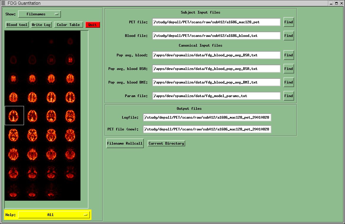
The first menu you encounter manages the filenames needed by this program. Four files are required by SPW_FDG. Two of these are standard files that are the same for every analysis and are stored in SPAMALIZE's data directory ("Pop avg. blood" and "Param files"). The other two files are the raw PET data ("PET file") and the blood file ("Blood file"). You will be unable to proceed to any of the other menus until you indicate valid filenames for each of these four data sources. The remaining two input files are required if you intend to scale a population-average blood TAC using data from the current subject.
Before you
can do anything else, you need to find the PET data. Most of the buttons are de-sensitized until a PET file has been
successfully read in. Select the "Find" button in the Filename menu
next to the PET filename box. Browse through your menu system until you find a
GE/Advance data file. Double-click on the file or select "OK" in the
browser menu. A menu for reading GE/Advance files will appear. Select the
button, "Read all Images in Data Set", unless for some reason you
only want a subset of the images. You can select any combination of images with
the file selection menu, but if you do this you are on your own!
At this point, SPW_FDG will read the PET data and store it all in memory (RAM). This implies you need to be working on a computer with enough RAM to store the entire PET file, which these days is not uncommon. You will get complaints if you cannot read the file, if the file is not a GE/Advance PET file, etc. You must fix any complaints before proceeding. Upon reading in your data, the first frame will be displayed at the left of the menu. If the images appear as salt-and-pepper noise, there was a byte-swapping problem you will have to fix.
SPW_FDG will
then search for a blood-file in the same directory as the PET scan. It will
look for a file named "a1234_blood.txt" or "a1234",
where
"1234" corresponds to the PET scan number contained in the PET
filename. If this file cannot be
located, SPW_FDG will then look for the blood file in a directory designated as
"blood_tac_dir" in the file
"/.../spamalize/data/spamalize_defaults_XXX.txt".
At the LfAN
this directory is currently /gig/blood/, and is used only for compatibility
with older protocols. Do not use this directory for new protocols! If the blood file still cannot be located,
you will have to browse for it. You may
also browse for and select an alternate blood file after the default file has
been located. This is how you would use a blood file you had created from a
previous session in SPW_FDG.
The standard files contain the population-average blood curve and the FDG model kinetic parameters. You may browse for and select alternate files if you wish. If the files are not suitable, SPW_FDG will complain when you try to move to the Blood File menu.
You can check
to see if the input files exist and are readable (by you!) by clicking on the
"Filename Rollcall" button in the Filename menu. This also checks the
validity of the output files, e.g. if one if the output files currently exist,
and you have write-permission for the designated directory. Copious checking is performed at each step
of the analysis to make sure the files have the correct format, that the values
make sense, etc., in an attempt to keep you out of trouble. If your data are
OK, you will not even notice any of these background checks.
B.
Blood TAC Menu
This menu
displays the values from the blood-file relevant to creating a time-activity
curve (TAC). The goal is to create a TAC with 1-second increments (sometimes
referred to as a 1-second grid) suitable for use with the PET data. This means
that the blood and PET units must be the same, decay-correction must correspond, etc.
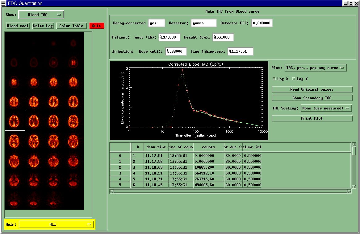
You may edit several of the values in the top window. The values that have an effect are:
- Decay-corrected: if "yes", indicates that the blood data have already been decay-corrected to the Injection time.
- Detector Eff: This is the detector efficiency, defined as the ratio of
- Time (hh.mm.ss): This is the injection time. If you need to change this, you should change the value in
- Patient Height (cm)
- Patient mass (lb.)
The other
values in the top menu are for informational purposes only.
The table at the bottom of this menu displays the blood values from the blood file. You may edit these if you wish. To do so, you must double-click on the desired cell. If the first entry in the blood-file has a draw-time after the injection time, a row is inserted at the beginning of the table with counts=0 and a draw time equal to the injection time. Attempts to change the draw-time in this row will be rebuffed- do not try this!
The Plot-window in the middle displays the measured blood points (red "plus" sign), the population-average curve scaled to the last measured blood value (green dots), and the resulting 1-sec gridded TAC (pink dots). There should be a smooth transition between the measured and population-average TAC at the last measured blood point. The dropdown menu "Plot" lets you examine each of the components individually.
You can import a secondary blood file to compare its TAC to your current TAC by selecting the "Show Secondary TAC" button. This is useful if you have two TACs from the same subject and you want to compare them to see if you may have missed an important time-point in the peak region. You may also use the Blood Tool for this.
Changing ANY of the values mentioned above (subject info or blood data) causes a new TAC to be calculated. The TAC you see displayed will definitely be the TAC that is used for producing the metabolic PET images. If you make some changes you are unsure of, you can read the original blood data by selecting the "Read Original Data" button. This (naturally) will result in a new TAC.
You can
easily create a new blood file with any changes you made by selecting the
"Write Log" button from the left-hand menu. The current blood values
are placed into one of the sections in the resulting text log-file, and can be
copied and pasted into a new file and used, as-is, for subsequent analysis.
Population-average scaled TAC:
There are several choices for scaling the TAC. The default is "None (use measured)", which means that the data contained in the blood file will be placed into the blood table, and any changes made to the blood table will be incorporated into the final TAC. No scaling performed with this option.
Not infrequently, there are problems with the blood data. The most common problem is that, due to technical problems with drawing the blood, the peak of the blood curve is insufficiently measured. If this occurs, all is not lost! To the contrary, there are several ways to estimate the blood curve using a scaled population-average TAC. Spamalize's FDG Tool gives you options to scale the population-average TAC according to:
- one or more accurate and reliable samples.
- the subject's Body-Surface-Area (BSA)
- the Body-Mass-Index (BMI).
These are listed in decreasing order of desireability. The downside to using a population-averaged scaled TAC is that if the subject at hand has a true blood TAC that differs greatly from the population-average, the quantitation will be suboptimal. Another repercussion is that you can only find the "influx constant", Ki, and you cannot attempt to find the individual rate constants (k1 - k4), but this is beyond the scope of SPW_FDG.
The best scaling approach is to use reliable blood data from the subject at hand, usually obtained later than 10 minutes post-injection. If you only have one blood sample, take it at 15 or 20 minutes. Otherwise, you can use all of the samples from 10 minutes post-injection and later. To do this, simply edit the blood table to set all of the sample counts you DO NOT wish to use to 0. Then select "Scale Measured" from the "TAC Scaling" menu, and the population-average curve will be scaled to match the remaining points. You may then proceed to subsequent menus, and the scaled population-average curve will be used to quantitate the PET data. The altered blood data will be written to the log-file, and the log-file will also contain a line detailing the scaling method that was used.
If you do not have any reliable blood points, all is not lost! You can also scale the population-average curve to the subject's Body Surface Area (BSA) or Body Mass Index (BMI). The BSA incorporates the injected dose and subject's weight and height, while the BMI is similar but does not require the height. Using the BSA gives a more accurate estimate of various body types, particularly if the subject does not have a strictly average body type. You should the BSA approach if possible, but sometimes the subject's height information was not recorded.
C.
Kinetic Model
This menu
shows:
- parameters for the FDG 3-compartment model;
- the resulting estimates of the
concentration in each compartment;
- the lCMRglu values for a single specified
PET value.
This is a
rich menu, enabling you to investigate various aspects of your data. This can
be particularly useful if you want to see the effect on lCMRglu due to small
changes in the blood data.
The top
portion contains the rate constants for this model. The rate constants,
designated as k1-k4, govern how much radioactivity passes from one compartment
to another in a given time. For instance, k1 governs what fraction of the
plasma radioactivity passes from the blood and into the tissue in 1 minute.
Likewise, k3 governs the fraction of
FDG in the
tissue that is metabolized into 6-P-FDG in one minute. Since FDG competes with
glucose, we need to know the (non-radioactive) glucose level in the plasma.
There are usually 3 glucose values, measured throughout the course of the
uptake of radioactivity.
The bottom
menu shows information for the current PET frame, and summarizes the average,
minimum, maximum, etc. values for this frame. You can investigate different
frames by typing the desired number in the "Frame" box, or by
clicking at the corresponding time in the plot-window.
The
"Model results" menu shows the lCMRglu value that results from using
the current specified PET value, Ci(T), for a time T which usually corresponds
to the middle of the current PET frame. In this menu, Ci(T) is a SINGLE
representative value. It is usually the average PET value for pixels above the
threshold, but you can type in any value you want.
Ce(T) and
Cm(T) show, respectively, the values calculated from the model at the time T
for the concentration of radioactive unmetabolized FDG and metabolized 6-P-FDG
in the tissue. You can change the values for T and Ci(T) by typing in their
text-box, or select the time T by clicking in the plot-window. If you select a
time T that is within the
current PET
frame, the time is automatically set to the middle of the frame. The value of
Ci(T) is frequently updated to correspond to the average PET value above the
indicated threshold for the current PET frame. The time duration of the current
PET frame is indicated by a green rectangle in the plot window. Other PET time
frames are indicated by vertical blue lines. The current time is indicated by a
vertical red line.
The image in
the bottom menu shows a single plane, usually the central one. You may display
other planes by clicking on the desired image in the left-hand window. The
white outline indicates the location of the threshold values used to calculate
the average value.
You can view
a histogram of the current raw PET image by selecting "Histogram of
Image" from the Plot pulldown menu. Click on the histogram to move the
threshold (not the average value!) to the current location.
D.
Metabolic Images
This menu
displays the metabolic PET images. To save your work, select the "Write
Metabolic Images" button. Note that the metabolic images are NOT
automatically written- you must select this button! In order to change the name
of the PET file, you must start over at the Filename Menu.
The metabolic
images shown in this menu can be compared to the original raw PET images.
Clicking in either of the "en masse" display windows will cause a
larger version of that particular image to be displayed on the right-hand side.
By moving the cursor over the single-slice images you can see the location and
values for both the raw and metabolic images. Clicking on either of the images
will place a crosshair, which can be convenient for comparing locations.
The threshold
here is the same percentage value as for the raw images, but the average value
will not correspond to the lCMRglu in the FDG Model menu, since there the
average refers to the average raw value, and here it refers to the average
metabolic rate value.
A.
Overview
Two files are
produced for each analysis:
1) An ANALYZE
file containing the metabolic PET data;
2) An
ASCII-text log-file containing a record of the parameters used and the actions
taken.
The rollcall
procedure checks to make sure that you have write- permission in the desired
output directory, that the disk is not full, and that the desired filename does
not already exist. If the file does exist, you will be asked if you want to
over-write the existing file. If you answer "No", a modified filename
will be suggested.
The ANALYZE
file actually consists of two (2) files, an image file (with extension .img)
and a header file (with extension .hdr). If you copy the PET data to another
directory, make sure to copy both the .img file and the .hdr file, or else you
will be unable to use your quantitated PET data!
The log-file
generally has a similar name as the ANALYZE PET file. Both output filenames
normally incorporate a date/time stamp, so you will have to work pretty hard to
overwrite existing data. On the other hand, if you run this program several
times in a row, you will have created a large number of files...
B.
Printing Data
You can send
most of the plots and most of the images to a color printer via the
"Print..." buttons sprinkled throughout the GUI. To use these, you must
make sure that SPW_FDG knows how to talk to your color printer.
If you are on
a unix computer, the printer commands must be set correctly in the SPAMALIZE
defaults file,
/.../spamalize/data/spamalize_defaults_unix.txt
If you are
using a non-unix computer (PC/Windows98, MacIntosh, etc.) you will be prompted
to browse for the desired computer. You should use a color printer if one is
available.
The log-file
is a simple text file and can be printed using any common text-editor, or with
simple printer commands.
C.
Log File
The logfile
contains all of the parameters that were actually used to calculate the
metabolic images. Note these values may not be the same as the values
originally in the blood and model data files, since you have the opportunity to
change them within SPW_FDG.
For each frame, a series of parameters (min, max, avg, etc.) are given for the raw data and for the metabolic data, along with their units and a typical range of values. The ranges are fairly liberal, so if any of your values fall outside of its corresponding range you should investigate why. Frequently there will be a simple reason (the person was very large so the radioactivity concentration was lower, the scan did not begin until 2 hours after injection, etc.), but occasionally