Introduction

Based on the Weighted Fourier Series (WFS) framework originally developed for brain cortical surfaces [1] and amygdala surfaces [2], white fiber tracks are parameterized using the cosine basis functions. This is a general framework for representing, registering and smoothing anatomical objects in a unified Hilbert space formulation. The cosine series representation for 3D curves is introduced in [3] and [5]. The implementation is based on MATLAB 7.5 and a Mac-OSX. If you are using the codes or data below, please reference [3] or [5]

Loading tract data to MATLAB  

Using the second order Runge-Kutta streamline algorithm with tensor deflection (TEND) [4], we obtained the whole brain tracts (001_spd_tracts.Bfloat.zip) for a single subject. You can use CAMINO package to obtain tracts. The complete MATLAB package excluding the tract data is zipped into cosine-representation.zip. After unzipping, load the tract.  The variable  SL consists of 10000 tracts and 1000-th tract can be displayed:

SL=get_streamlines('001_spd_tracts.Bfloat',[1.5 1.75 2.25]);
tract=SL{1000}';
figure; plot3(tract(1,:),tract(2,:),tract(3,:),'.b') 

Cosine series representation

The parameterization of the tract is done by

[arc_length  para]=parameterize_arclength(tract);

Note that this is not the arclengh paramterization. Instead we paramterize the arclength as a unit interval. The i-th control point in the tract tract(:,i)is mapped to para(i), where para is a number between 0 and 1:

figure;
subplot(3,1,1); plot(para, tract(1,:));
subplot(3,1,2); plot(para, tract(2,:));
subplot(3,1,3); plot(para, tract(3,:));

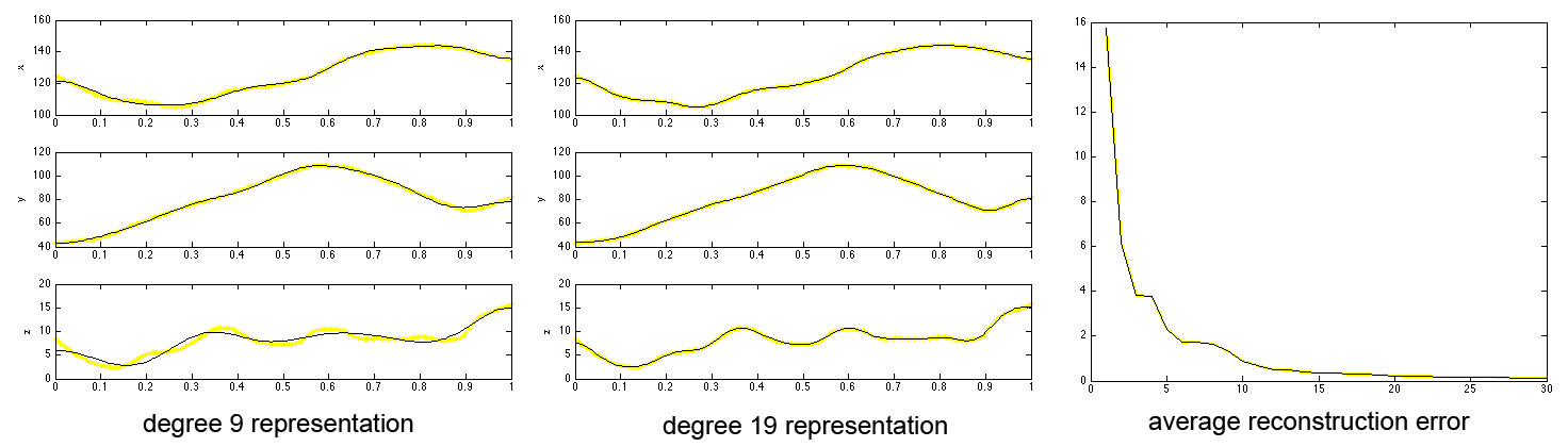
Figure 1. Plots of x,y,z coordinates of the cosine series representation. Yellow lines are the original tract coordinates (tract) and black lines (wfs) are the reconstruction. The average reconstruction error over degree is given in terms of mean sum of squared errors over whole tract. See [3] for detail.

The 19-th degree cosine series representation is given by

[wfs beta]=WFS_tracts(tract,para,19);
figure; plot3(tract(1,:),tract(2,:),tract(3,:),'.y') %original data
hold on; plot3(wfs(:,1),wfs(:,2),wfs(:,3),'-k') %reconstruction

beta is the estimated Fourier coefficients and wfs is the coordinates of the representation.

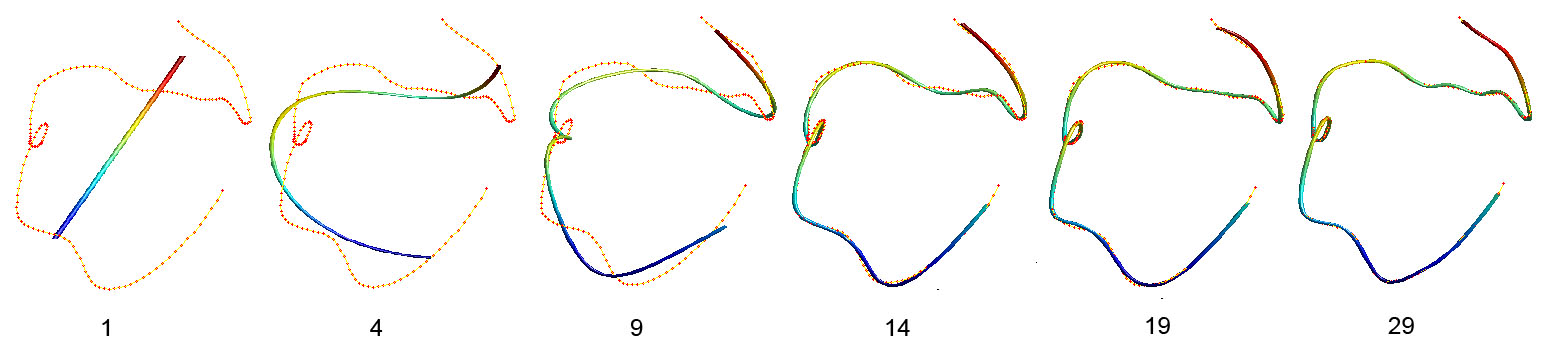
Figure 2. The cosine series representation at various degrees. The orange dots are variable tract while the colored lines are variable wfs.

Averaging curves

The cosine series representation can be used to average the collection of curves by simply averaging the coefficients. Consider another tract generated by adding noise:

tract2 = tract + normrnd(0,0.5,3,491);
hold on; plot3(tract2(1,:),tract2(2,:),tract2(3,:),'.y')

[arc_length2  para2]=parameterize_arclength(tract2);
[wfs2 beta2]=WFS_tracts(tract2,para2,19);
hold on; plot3(wfs2(:,1),wfs2(:,2),wfs2(:,3),'-k') %reconstruction

It is nonsense to simply average tract and tract2 by averaging their coordinates. Instead, we simply average the representation. Using the average coefficients, we can reconstruct the cosine representation using WFS_resample.

beta_a= (beta + beta2)/2;
para_a = [1:200]/200;
wfs_a=WFS_resample(beta_a,19, para_a);
hold on; plot3(wfs_a(:,1),wfs_a(:,2),wfs_a(:,3),'-r')

Simulating 3D curves

This is an example given in [3]. Taking this as the underlying signal, noises are added nonlinaerly to obtain the simulation results.

t=0:0.1:10
tract=[t.*sin(t); t.*cos(t); t];
figure; plot3(tract(1,:),tract(2,:),tract(3,:),'.b') %simulation

[arc_length  para]=parameterize_arclength(tract);
[wfs beta]=WFS_tracts(tract,para,19);
hold on; plot3(wfs(:,1),wfs(:,2),wfs(:,3),'r') %reconstruction

Streamtube representation

Figure 7 in paper [3] has a very interesting visualization technique called the streamtube representation. This is done using the built-in function called streamtube in MATLAB.

figure; figure_streamtube(tract', 0.5, [1 .3 .3]);
camlight

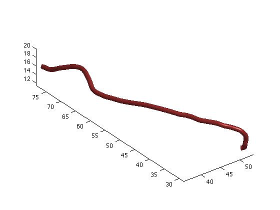
Figure 3. The streamtube representation of a tract.

This generates Figure 3. If you use this function multiple times while holding the figure using the hold on command,  you can generate some amazing 3D tract visualization (Figure 4).

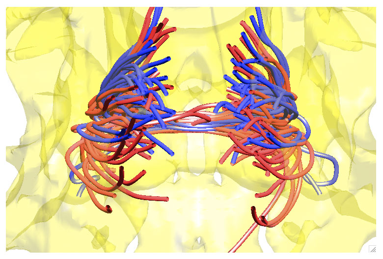
Figure 4. The streamtube representation of a bundle of tracts for two groups (red= autism, blue = controls). See paper [3] for details.

Weighted Fourier series (WFS) representation

The terms in the cosine series representation can be exponentially weighted in such a way that the expansion is the solution of heat diffusion or equivalently heat kernel smoothing. For details, see [1].
We will demonstrate this using EEG time series published in [6]. The representation can be used to smooth out noisy EEG (Figure 5).

 load EEG.mat
x=[1:3500]/3500;
k=2000;
sigma=0.0001;
[wfs beta]=WFS_COSINE(EEG(1,:)',x',k,sigma);
figure; plot(EEG(1,:), '.k');
hold on; plot(wfs, 'r', 'linewidth',1)

Figure 5. Weighted Fourier series representation of EEG, which is equivalent to heat diffusion. Left is with bandwidth 0.00001 and right is with bandwidth 0.0001.

References

[1] Chung, M.K., Dalton, K.M., Shen, L., L., Evans, A.C., Davidson, R.J. 2007. Weighted Fourier series representation and its application to quantifying the amount of gray matter. IEEE Transactions on Medical Imaging 26:566-581.

[2] Chung, M.K. Nacewicz, B.M., Wang, S., Dalton, K.M., Pollak, S., Davidson, R.J. 2008. Amydala surface modeling with weighted spherical harmonics. 4th International Workshop on Medical Imaging and Augmented Reality (MIAR). Lecture Notes in Computer Sciences (LNCS) 5128:177-184.

[3] Chung, M.K. Adluru, N., Lee, J.E., Lazar, M., Lainhart, J.E., Alexander, A.L. 2010. Cosine series representation of 3D curves and its application to white matter fiber bundles in diffusion tensor imaging. Statistics and Its Interface  3:69-80.

[4] Lazar, M., Alexander, A.L. 2005. Bootstrap white matter tractography (BOOT-TRAC). NeuroImage 24:524-532.

[5] Chung, M.K. 2013. Statistical and Computational Methods in Brain Image Analysis.  CRC Press. DATA/MATLAB. The detail is given in Chapter 10.

[6] Wang, Y., Chung, M., Bachhuber, D.R.W., Schaefer, S.M., van Reekum, C.M., Davidson, R.J. 2015 LARS network filtration in the study of EEG brain connectivity, IEEE 12th International Symposium on Biomedical Imaging (ISBI) 30-33